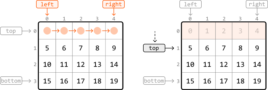
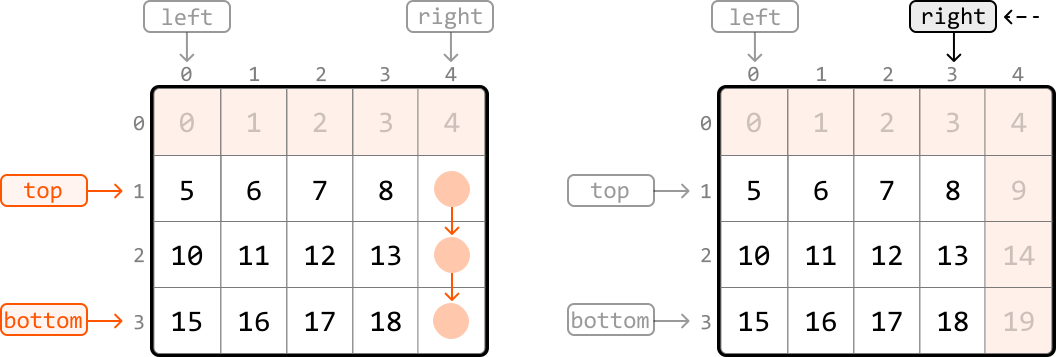
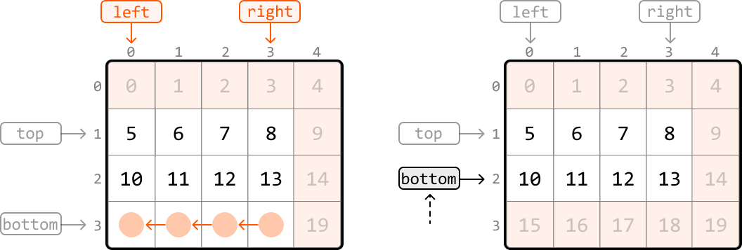
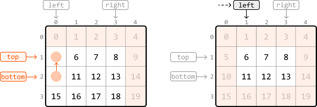
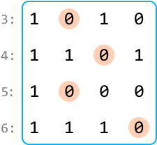
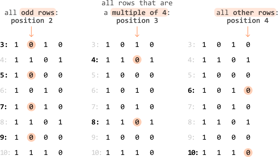
As the name implies, a two-pointer pattern refers to an algorithm that utilizes two pointers. But what is a pointer? It's a variable that represents an index or position within a data structure, like an array or linked list. Many algorithms just use a single pointer to attain or keep track of a single element:
Introducing a second pointer opens a new world of possibilities. Most importantly, we can now make comparisons. With pointers at two different positions, we can compare the elements at those positions and make decisions based on the comparison:
In many cases, such comparisons are made using two nested for-loops, which takes O(n2) time, where n denotes the length of the data structure. In the code snippet below, i and j are two pointers used to compare every two elements of an array:
for i in range(n):
    for j in range(i + 1, n):
        compare(nums[i], nums[j])
for (let i = 0; i < n; i++) {
    for (let j = i + 1; j < n; j++) {
        compare(nums[i], nums[j]);
    }
}
for (int i = 0; i < n; i++) {
    for (int j = i + 1; j < n; j++) {
        compare(nums[i], nums[j]);
    }
}
Often, this approach does not take advantage of predictable dynamics that might exist in a data structure. An example of a data structure with predictable dynamics is a sorted array: when we move a pointer in a sorted array, we can predict whether the value being moved to is greater or smaller. For example, moving a pointer to the right in an ascending array guarantees we're moving to a value greater than or equal to the current one:
As you can see, data structures with predictable dynamics let us move pointers in a logical way. Taking advantage of this predictability can lead to improved time and space complexity, which we will illustrate with real interview problems in this chapter.
Two-pointer Strategies
Two-pointer algorithms usually take only O(n) time by eliminating the need for nested for-loops. There are three main strategies for using two pointers.
Inward traversal
This approach has pointers starting at opposite ends of the data structure and moving inward toward each other:
The pointers move toward the center, adjusting their positions based on comparisons, until a certain condition is met, or they meet/cross each other. This is ideal for problems where we need to compare elements from different ends of a data structure.
Unidirectional traversal
In this approach, both pointers start at the same end of the data structure (usually the beginning) and move in the same direction:
These pointers generally serve two different but supplementary purposes. A common application of this is when we want one pointer to find information (usually the right pointer) and another to keep track of information (usually the left pointer).
Staged traversal
In this approach, we traverse with one pointer, and when it lands on an element that meets a certain condition, we traverse with the second pointer:
Similar to unidirectional traversal, both pointers serve different purposes. Here, the first pointer is used to search for something, and once found, a second pointer finds additional information concerning the value at the first pointer.
We discuss all of these techniques in detail throughout the problems in this chapter.
When To Use Two Pointers?
A two-pointer algorithm usually requires a linear data structure, such as an array or linked list. Otherwise, an indication that a problem can be solved using the two-pointer algorithm, is when the input follows a predictable dynamic, such as a sorted array.
Predictable dynamics can take many forms. Take, for instance, a palindromic string. Its symmetrical pattern allows us to logically move two pointers toward the center. As you work through the problems in this chapter, you'll learn to recognize these predictable dynamics more easily.
Another potential indicator that a problem can be solved using two pointers is if the problem asks for a pair of values or a result that can be generated from two values.
Real-world Example
Garbage collection algorithms: In memory compaction – which is a key part of garbage collection – the goal is to free up contiguous memory space by eliminating gaps left by deallocated (aka dead) objects. A two-pointer technique helps achieve this efficiently: a 'scan' pointer traverses the heap to identify live objects, while a 'free' pointer keeps track of the next available space to where live objects should be relocated. As the 'scan' pointer moves, it skips over dead objects and shifts live objects to the position indicated by the 'free' pointer, compacting the memory by grouping all live objects together and freeing up continuous blocks of memory.
Chapter Outline
The two-pointer pattern is very versatile and, consequently, quite broad. As such, we want to cover more specialized variants of this algorithm in separate chapters, such as Fast and Slow Pointers and Sliding Windows.
CHAPTER 02
Pair Sum - Sorted
Given an array of integers sorted in ascending order and a target value, return the indexes of any pair of numbers in the array that sum to the target. The order of the indexes in the result doesn't matter. If no pair is found, return an empty array.
Explanation: other valid outputs could be [1, 0], [0, 2], [2, 0], [1, 2] or [2, 1].
Intuition
The brute force solution to this problem involves checking all possible pairs. This is done using two nested loops: an outer loop that traverses the array for the first element of the pair, and an inner loop that traverses the rest of the array to find the second element. Below is the code snippet for this approach:
from typing import List

def pair_sum_sorted_brute_force(nums: List[int], target: int) -> List[int]:
    n = len(nums)
    for i in range(n):
        for j in range(i + 1, n):
            if nums[i] + nums[j] == target:
                return [i, j]
    return []
function pairSumSortedBruteForce(nums, target) {
    const n = nums.length;
    for (let i = 0; i < n; i++) {
        for (let j = i + 1; j < n; j++) {
            if (nums[i] + nums[j] === target) {
                return [i, j];
            }
        }
    }
    return [];
}
public int[] pairSumSortedBruteForce(int[] nums, int target) {
    int n = nums.length;
    for (int i = 0; i < n; i++) {
        for (int j = i + 1; j < n; j++) {
            if (nums[i] + nums[j] == target) {
                return new int[]{i, j};
            }
        }
    }
    return new int[]{};
}
This approach has a time complexity of O(n2), where n denotes the length of the array. This approach does not take into account that the input array is sorted. Could we use this fact to come up with a more efficient solution?
A two-pointer approach is worth considering here because a sorted array allows us to move the pointers in a logical way. Let's see how this works in the example below:
A good place to start is by looking at the smallest and largest values: the first and last elements, respectively. The sum of these two values is 1.
Since 1 is less than the target, we need to move one of our pointers to find a new pair with a larger sum.
Left pointer: The left pointer will always point to a value less than or equal to the value at the right pointer because the array is sorted. Incrementing it would result in a sum greater than or equal to the current sum of 1.
Right pointer: Decrementing the right pointer would result in a sum that’s less than or equal to 1.
Therefore, we should increment the left pointer to find a larger sum:
Again, the sum of the values at those two pointers (4) is too small. So, let's increment the left pointer:
Now, the sum (9) is too large. So, we should decrement the right pointer to find a pair of values with a smaller sum:
Finally, we found two numbers that yield a sum equal to the target. Let’s return their indexes:
Above, we’ve demonstrated a two-pointer algorithm using inward traversal. Let’s summarize this logic. For any pair of values at left and right:
If their sum is less than the target, increment left, aiming to increase the sum towards the target value.
If their sum is greater than the target, decrement right, aiming to decrease the sum towards the target value.
If their sum is equal to the target value, return [left, right].
We can stop moving the left and right pointers when they meet, as this indicates no pair summing to the target was found.
Try it yourself
Write your solution to the problem before checking the reference implementation.
Implementation
from typing import List

def pair_sum_sorted(nums: List[int], target: int) -> List[int]:
    left, right = 0, len(nums) - 1
    while left < right:
        sum = nums[left] + nums[right]
        # If the sum is smaller, increment the left pointer, aiming to increase the
        # sum towards the target value.
        if sum < target:
            left += 1
        # If the sum is larger, decrement the right pointer, aiming to decrease the
        # sum towards the target value.
        elif sum > target:
            right -= 1
        # If the target pair is found, return its indexes.
        else:
            return [left, right]
    return []
function pairSumSorted(nums, target) {
    let left = 0, right = nums.length - 1;
    while (left < right) {
        const sum = nums[left] + nums[right];
        // If the sum is smaller, increment the left pointer, aiming to increase the
        // sum towards the target value.
        if (sum < target) {
            left++;
        // If the sum is larger, decrement the right pointer, aiming to decrease the
        // sum towards the target value.
        } else if (sum > target) {
            right--;
        // If the target pair is found, return its indexes.
        } else {
            return [left, right];
        }
    }
    return [];
}
public int[] pairSumSorted(int[] nums, int target) {
    int left = 0, right = nums.length - 1;
    while (left < right) {
        int sum = nums[left] + nums[right];
        // If the sum is smaller, increment the left pointer, aiming to increase the
        // sum towards the target value.
        if (sum < target) {
            left++;
        // If the sum is larger, decrement the right pointer, aiming to decrease the
        // sum towards the target value.
        } else if (sum > target) {
            right--;
        // If the target pair is found, return its indexes.
        } else {
            return new int[]{left, right};
        }
    }
    return new int[]{};
}
Complexity Analysis
Time complexity: The time complexity of pair_sum_sorted is O(n) because we perform approximately n iterations using the two-pointer technique in the worst case.
Space complexity: We only allocated a constant number of variables, so the space complexity is O(1).
Test Cases
In addition to the examples already discussed, here are some other test cases you can use. These extra test cases cover different contexts to ensure the code works well across a range of inputs. Testing is important because it helps identify mistakes in your code, ensures the solution works for uncommon inputs, and brings attention to cases you might have overlooked.
Input
Expected output
Description
nums = [] target = 0
[]
Tests an empty array.
nums = [1] target = 1
[]
Tests an array with just one element.
nums = [2, 3] target = 5
[0, 1]
Tests a two-element array that contains a pair that sums to the target.
nums = [2, 4] target = 5
[]
Tests a two-element array that doesn’t contain a pair that sums to the target.
nums = [2, 2, 3] target = 5
[0, 2] or [1, 2]
Testing an array with duplicate values.
nums = [-1, 2, 3] target = 2
[0, 2]
Tests if the algorithm works with a negative number in the target pair.
nums = [-3, -2, -1] target = -5
[0, 1]
Tests if the algorithm works with both numbers of the target pair being negative.
Interview Tip
Tip: Consider all information provided.
When interviewers pose a problem, they sometimes provide only the minimum amount of information required for you to start solving it. Consequently, it’s crucial to thoroughly evaluate all that information to determine which details are essential for solving the problem efficiently. In this problem, the key to arriving at the optimal solution is recognizing that the input is sorted.
CHAPTER 03
Triplet Sum
Given an array of integers, return all triplets [a, b, c] such that a + b + c = 0 . The solution must not contain duplicate triplets (e.g., [1, 2, 3] and [2, 3, 1] are considered duplicates). If no such triplets are found, return an empty array.
Each triplet can be arranged in any order, and the output can be returned in any order.
A brute force solution involves checking every possible triplet in the array to see if they sum to zero. This can be done using three nested loops, iterating through each combination of three elements.
Duplicate triplets can be avoided by sorting each triplet, which ensures that identical triplets with different representations (e.g., [1, 3, 2] and [3, 2, 1]) are ordered consistently (e.g., [1, 2, 3]). Once sorted, we can add these triplets to a hash set. This way, if the same triplet is encountered again, the hash set will only keep one instance. Below is the code snippet for this approach:
from typing import List

def triplet_sum_brute_force(nums: List[int]) -> List[List[int]]:
    n = len(nums)
    # Use a hash set to ensure we don't add duplicate triplets.
    triplets = set()
    # Iterate through the indexes of all triplets.
    for i in range(n):
        for j in range(i + 1, n):
            for k in range(j + 1, n):
                if nums[i] + nums[j] + nums[k] == 0:
                    # Sort the triplet before including it in the hash set.
                    triplet = tuple(sorted([nums[i], nums[j], nums[k]]))
                    triplets.add(triplet)
    return [list(triplet) for triplet in triplets]
function tripletSumBruteForce(nums) {
    const n = nums.length;
    // Use a hash set to ensure we don't add duplicate triplets.
    const triplets = new Set();
    // Iterate through the indexes of all triplets.
    for (let i = 0; i < n; i++) {
        for (let j = i + 1; j < n; j++) {
            for (let k = j + 1; k < n; k++) {
                if (nums[i] + nums[j] + nums[k] === 0) {
                    // Sort the triplet before including it in the hash set.
                    const triplet = [nums[i], nums[j], nums[k]].sort((a, b) => a - b);
                    triplets.add(JSON.stringify(triplet));
                }
            }
        }
    }
    return Array.from(triplets, item => JSON.parse(item));
}
public List<List<Integer>> tripletSumBruteForce(int[] nums) {
    int n = nums.length;
    // Use a hash set to ensure we don't add duplicate triplets.
    Set<List<Integer>> triplets = new HashSet<>();
    // Iterate through the indexes of all triplets.
    for (int i = 0; i < n; i++) {
        for (int j = i + 1; j < n; j++) {
            for (int k = j + 1; k < n; k++) {
                if (nums[i] + nums[j] + nums[k] == 0) {
                    // Sort the triplet before including it in the hash set.
                    List<Integer> triplet = Arrays.asList(nums[i], nums[j], nums[k]);
                    Collections.sort(triplet);
                    triplets.add(triplet);
                }
            }
        }
    }
    return new ArrayList<>(triplets);
}
This solution is quite inefficient with a time complexity of O(n3), where n denotes the length of the input array. How can we do better?
Let’s see if we can find at least one triplet that sums to 0. Notice that if we fix one of the numbers in a triplet, the problem can be reduced to finding the other two. This leads to the following observation:
For any triplet [a, b, c], if we fix 'a', we can focus on finding a pair [b, c] that sums to '-a' (a + b + c = 0 → b + c = -a).
Sound familiar? That's because the problem of finding a pair of numbers that sum to a target has already been addressed by Pair Sum - Sorted. However, we can only use that algorithm on a sorted array. So, the first thing we should do is sort the input. Consider the following example:
Now, starting at the first element, -2 (i.e., 'a'), we'll use the pair_sum_sorted method on the rest of the array to find a pair whose sum equals 2 (i.e., '-a'):
As you can see, when we called pair_sum_sorted, we did not find a pair with a sum of 2. This indicates that there are no triplets starting with -2 that add up to 0.
So, let's increment our main pointer, i, and try again.
This time, we found one pair that resulted in a valid triplet.
If we continue this process for the rest of the array, we find that [-1, -1, 2] is the only triplet whose sum is 0.
There’s an important difference between the pair_sum_sorted implementation in Pair Sum - Sorted and the one in this problem: for this problem, we don’t stop when we find one pair, we keep going until all target pairs are found.
Handling duplicate triplets
Something we previously glossed over is how to avoid adding duplicate triplets. There are two cases in which this happens. Consider the example below:
Case 1: duplicate ‘a’ values
The first instance where duplicates may occur is when seeking pairs for triplets that start with the same ‘a’ value:
Since pair_sum_sorted would look for pairs that sum ‘-a’ in both instances, we’d naturally end up with the same pairs and, hence, the same triplets.
To avoid picking the same 'a' value, we keep increasing i (where num[i] represents the value 'a') until it reaches a different number from the previous one. We do this before we start looking for pairs using the pair_sum_sorted method. This logic works because the array is sorted, meaning equal numbers are next to each other. The code snippet for checking duplicate 'a' values looks like this:
# To prevent duplicate triplets, ensure 'a' is not a repeat of the previous element
# in the sorted array.
if i > 0 and nums[i] == nums[i - 1]:
    continue
... Find triplets ...
// To prevent duplicate triplets, ensure 'a' is not a repeat of the previous element
// in the sorted array.
if (i > 0 && nums[i] === nums[i - 1]) {
    continue;
}
// ... Find triplets ...
// To prevent duplicate triplets, ensure 'a' is not a repeat of the previous element
// in the sorted array.
if (i > 0 && nums[i] == nums[i - 1]) {
    continue;
}
// ... Find triplets ...
Case 2: duplicate ‘b’ values
As for the second case, consider what happens during pair_sum_sorted when we encounter a similar issue. For a fixed target value (‘-a’), pairs that start with the same number ‘b’ will always be the same:
The remedy for this is the same as before: ensure the current ‘b’ value isn’t the same as the previous value.
It’s important to note that we don’t need to explicitly handle duplicate 'c' values. The adjustments made to avoid duplicate 'a' and 'b' values ensure each pair [a, b] is unique. Since 'c' is determined by the equation c = -(a + b), each unique [a, b] pair will result in a unique 'c' value. Therefore, by just avoiding duplicates in 'a' and 'b', we automatically avoid duplicates in the [a, b, c] triplets.
Optimization
An interesting observation is that triplets that sum to 0 cannot be formed using positive numbers alone. Therefore, we can stop trying to find triplets once we reach a positive ‘a’ value since this implies that ‘b’ and ‘c’ would also be positive.
Try it yourself
Write your solution to the problem before checking the reference implementation.
Implementation
From the above intuition, we know we need to slightly modify the pair_sum_sorted function to avoid duplicate triplets. We also need to pass in a start value to indicate the beginning of the subarray on which we want to perform the pair-sum algorithm. Otherwise, the two-pointer logic remains nearly identical to that of Pair Sum - Sorted.
from typing import List

def triplet_sum(nums: List[int]) -> List[List[int]]:
    triplets = []
    nums.sort()
    for i in range(len(nums)):
        # Optimization: triplets consisting of only positive numbers will never sum
        # to 0.
        if nums[i] > 0:
            break
        # To avoid duplicate triplets, skip 'a' if it's the same as the previous
        # number.
        if i > 0 and nums[i] == nums[i - 1]:
            continue
        # Find all pairs that sum to a target of '-a' ('-nums[i]').
        pairs = pair_sum_sorted_all_pairs(nums, i + 1, -nums[i])
        for pair in pairs:
            triplets.append([nums[i]] + pair)
    return triplets

def pair_sum_sorted_all_pairs(nums: List[int], start: int, target: int) -> List[int]:
    pairs = []
    left, right = start, len(nums) - 1
    while left < right:
        sum = nums[left] + nums[right]
        if sum == target:
            pairs.append([nums[left], nums[right]])
            left += 1 # To avoid duplicate '[b, c]' pairs, skip 'b' if it’s the same as the # previous number.
            while left < right and nums[left] == nums[left - 1]:
                left += 1
        elif sum < target:
            left += 1
        else:
            right -= 1
    return pairs
function tripletSum(nums) {
    const triplets = [];
    nums.sort((a, b) => a - b);
    for (let i = 0; i < nums.length; i++) {
        // Optimization: triplets consisting of only positive numbers will never sum
        // to 0.
        if (nums[i] > 0) {
            break;
        }
        // To avoid duplicate triplets, skip 'a' if it's the same as the previous
        // number.
        if (i > 0 && nums[i] === nums[i - 1]) {
            continue;
        }
        // Find all pairs that sum to a target of '-a' ('-nums[i]').
        const pairs = pairSumSortedAllPairs(nums, i + 1, -nums[i]);
        for (const pair of pairs) {
            triplets.push([nums[i], ...pair]);
        }
    }
    return triplets;
}

function pairSumSortedAllPairs(nums, start, target) {
    const pairs = [];
    let left = start, right = nums.length - 1;
    while (left < right) {
        const sum = nums[left] + nums[right];
        if (sum === target) {
            pairs.push([nums[left], nums[right]]);
            left++; // To avoid duplicate '[b, c]' pairs, skip 'b' if it’s the same as the previous number.
            while (left < right && nums[left] === nums[left - 1]) {
                left++;
            }
        } else if (sum < target) {
            left++;
        } else {
            right--;
        }
    }
    return pairs;
}
public List<List<Integer>> tripletSum(int[] nums) {
    List<List<Integer>> triplets = new ArrayList<>();
    Arrays.sort(nums);
    for (int i = 0; i < nums.length; i++) {
        // Optimization: triplets consisting of only positive numbers will never sum
        // to 0.
        if (nums[i] > 0) {
            break;
        }
        // To avoid duplicate triplets, skip 'a' if it's the same as the previous
        // number.
        if (i > 0 && nums[i] == nums[i - 1]) {
            continue;
        }
        // Find all pairs that sum to a target of '-a' ('-nums[i]').
        List<List<Integer>> pairs = pairSumSortedAllPairs(nums, i + 1, -nums[i]);
        for (List<Integer> pair : pairs) {
            triplets.add(Arrays.asList(nums[i], pair.get(0), pair.get(1)));
        }
    }
    return triplets;
}

public List<List<Integer>> pairSumSortedAllPairs(int[] nums, int start, int target) {
    List<List<Integer>> pairs = new ArrayList<>();
    int left = start, right = nums.length - 1;
    while (left < right) {
        int sum = nums[left] + nums[right];
        if (sum == target) {
            pairs.add(Arrays.asList(nums[left], nums[right]));
            left++; // To avoid duplicate '[b, c]' pairs, skip 'b' if it’s the same as the previous number.
            while (left < right && nums[left] == nums[left - 1]) {
                left++;
            }
        } else if (sum < target) {
            left++;
        } else {
            right--;
        }
    }
    return pairs;
}
Complexity Analysis
Time complexity: The time complexity of triplet_sum is O(n2). Here’s why:
We first sort the array, which takes O(nlog(n)) time.
Then, for each of the n elements in the array, we call pair_sum_sorted_all_pairs at most once, which runs in O(n) time.
Therefore, the overall time complexity is O(log(n))+O(n2)=O(n2).
Space complexity: The space complexity is O(n) due to the space taken up by Python’s sorting algorithm. It's important to note that this complexity does not include the output array triplets because we’re only concerned with the additional space used by the algorithm, not the space needed for the output itself.
If the interviewer asks what the space complexity would be if we included the output array, it would be O(n2). This is because the pair_sum_sorted_all_pairs function, in the worst case, can add approximately n pairs to the output. Since this function is called approximately n times, the overall space complexity is O(n2).
Test Cases
In addition to the examples already covered in this explanation, below are some others to consider when testing your code.
Input
Expected output
Description
nums = []
[]
Tests an empty array.
nums = [0]
[]
Tests a single-element array.
nums = [1, -1]
[]
Tests a two-element array.
nums = [0, 0, 0]
[0, 0, 0]
Tests an array where all three of its values are the same.
nums = [1, 0, 1]
[]
Tests an array with no triplets that sum to 0.
nums = [0, 0, 1, -1, 1, -1]
[-1, 0, 1]
Tests an array with duplicate triplets.
CHAPTER 04
Is Palindrome Valid
A palindrome is a sequence of characters that reads the same forward and backward.
Given a string, determine if it's a palindrome after removing all non-alphanumeric characters. A character is alphanumeric if it's either a letter or a number.
Example 1:
Example
Input: s = 'a dog! a panic in a pagoda.'
Output: True
Example 2:
Example
Input: s = 'abc123'
Output: False
Constraints:
The string may include a combination of lowercase English letters, numbers, spaces, and punctuations.
Intuition
Identifying palindromes
A string is a palindrome if it remains identical when read from left to right or right to left. In other words, if we reverse the string, it should still read the same, disregarding spaces and punctuation:
An important observation is that if a string is a palindrome, the first character would be the same as the last, the second character would be the same as the second-to-last, etc:
A palindrome of odd length is different because it has a middle character. In this case, the middle character can be ignored since it has no “mirror” character elsewhere in the string.
Palindromes provides an ideal scenario for using two pointers (left and right). By initially setting the pointers at the beginning and end of the string, we can compare the characters at these positions. Ignoring non-alphanumeric characters for the moment, the logic can be summarized as follows:
If the alphanumeric characters at left and right are the same, move both pointers inward to process the next pair of characters.
If not, the string is not a palindrome: return false.
If we successfully compare all character pairs without returning false, the string is a palindrome, and we should return true.
Processing non-alphanumeric characters
Now, let's explore how to find palindromes that include non-alphanumeric characters.
Since non-alphanumeric characters don’t affect whether a string is a palindrome, we should skip them. This can be achieved with the following approach, which ensures the left and right pointers are adjusted to focus only on alphanumeric characters:
Increment left until the character it points to is alphanumeric.
Decrement right until the character it points to is alphanumeric.
With this in mind, let’s check if the string below is a palindrome using all the information we know so far:
As shown above, when the left and right pointers meet, it signals our exit condition. When these pointers meet, we've reached the middle character of the palindrome, at which point we can exit the loop since the middle character doesn’t need to be evaluated. However, we need to keep in mind that exiting when left equals right won't always be sufficient as an exit condition. For example, if the number of alphanumeric characters is even, the pointers won’t meet. This can be observed below:
Therefore, we need to ensure we exit the loop when left equals right, or when left passes right. In other words, the algorithm continues while left is less than right:
Example
while left < right:
Try it yourself
Write your solution to the problem before checking the reference implementation.
Implementation
In Python, we can use the inbuilt isalnum method to check if a character is alphanumeric.
def is_palindrome_valid(s: str) -> bool:
    left, right = 0, len(s) - 1
    while left < right:
        # Skip non-alphanumeric characters from the left.
        while left < right and not s[left].isalnum():
            left += 1
        # Skip non-alphanumeric characters from the right.
        while left < right and not s[right].isalnum():
            right -= 1
        # If the characters at the left and right pointers don’t match, the string is
        # not a palindrome.
        if s[left] != s[right]:
            return False
        left += 1
        right -= 1
    return True
function isPalindromeValid(s) {
    const isAlnum = (ch) => /[a-zA-Z0-9]/.test(ch);
    let left = 0, right = s.length - 1;
    while (left < right) {
        // Skip non-alphanumeric characters from the left.
        while (left < right && !isAlnum(s[left])) {
            left++;
        }
        // Skip non-alphanumeric characters from the right.
        while (left < right && !isAlnum(s[right])) {
            right--;
        }
        // If the characters at the left and right pointers don’t match, the string is
        // not a palindrome.
        if (s[left] !== s[right]) {
            return false;
        }
        left++;
        right--;
    }
    return true;
}
public boolean isPalindromeValid(String s) {
    int left = 0, right = s.length() - 1;
    while (left < right) {
        // Skip non-alphanumeric characters from the left.
        while (left < right && !Character.isLetterOrDigit(s.charAt(left))) {
            left++;
        }
        // Skip non-alphanumeric characters from the right.
        while (left < right && !Character.isLetterOrDigit(s.charAt(right))) {
            right--;
        }
        // If the characters at the left and right pointers don’t match, the string is
        // not a palindrome.
        if (s.charAt(left) != s.charAt(right)) {
            return false;
        }
        left++;
        right--;
    }
    return true;
}
Complexity Analysis
Time complexity: The time complexity of is_palindrome_valid is O(n), where n denotes the length of the string. This is because we perform approximately n iterations using the two-pointer technique.
Space complexity: We only allocated a constant number of variables, so the space complexity is O(1).
Test Cases
In addition to the examples discussed, below are more examples to consider when testing your code.
Input
Expected output
Description
s = ""
True
Tests an empty string.
s = "a"
True
Tests a single-character string.
s = "aa"
True
Tests a palindrome with two characters.
s = "ab"
False
Tests a non-palindrome with two characters.
s = "!, (?)"
True
Tests a string with no alphanumeric characters.
s = "12.02.2021"
True
Tests a palindrome with punctuation and numbers.
s = "21.02.2021"
False
Tests a non-palindrome with punctuation and numbers.
s = "hello, world!"
False
Tests a non-palindrome with punctuation.
Interview Tips
Tip 1: Clarify problem constraints.
It's common to not receive all the details of a problem from an interviewer. For example, you might only be asked to "check if a string is a palindrome." But before diving into a solution, it's important to clarify details with the interviewer, such as the presence of non-alphanumeric characters, their treatment, the role of numbers, the case sensitivity of letters, and other relevant details.
Tip 2: Confirm before using significant in-built functions.
This problem is made easier by using in-built functions such as .isalnum (or equivalent). Before using an in-built function that simplifies the implementation, ask the interviewer if it's okay to use it, or if they would prefer you implement it yourself.
The interviewer will most likely allow the use of an in-built function, or ask you to implement it as an exercise for later in the interview. If you use an in-built function, make sure you understand its time and space complexity.
Remember that interviewers are looking for team players, and this shows them you're considerate of their preferences and can adapt your approach based on the requirements.
CHAPTER 05
Largest Container
You are given an array of numbers, each representing the height of a vertical line on a graph. A container can be formed with any pair of these lines, along with the x-axis of the graph. Return the amount of water which the largest container can hold.
Example:
Example
Input: heights = [2, 7, 8, 3, 7, 6]
Output: 24
Intuition
If we have two vertical lines, heights[i] and heights[j], the amount of water that can be contained between these two lines is min(heights[i], heights[j]) * (j - i), where j - i represents the width of the container. We take the minimum height because filling water above this height would result in overflow.
In other words, the area of the container depends on two things:
The width of the rectangle.
The height of the rectangle, as dictated by the shorter of the two lines.
The brute force approach to this problem involves checking all pairs of lines, and returning the largest area found between each pair:
from typing import List

def largest_container_brute_force(heights: List[int]) -> int:
   n = len(heights)
   max_water = 0
   # Find the maximum amount of water stored between all pairs of lines.
   for i in range(n):
       for j in range(i + 1, n):
           water = min(heights[i], heights[j]) * (j - i)
           max_water = max(max_water, water)
   return max_water
function largestContainerBruteForce(heights) {
    const n = heights.length;
    let maxWater = 0;
    // Find the maximum amount of water stored between all pairs of lines.
    for (let i = 0; i < n; i++) {
        for (let j = i + 1; j < n; j++) {
            const water = Math.min(heights[i], heights[j]) * (j - i);
            maxWater = Math.max(maxWater, water);
        }
    }
    return maxWater;
}
public int largestContainerBruteForce(int[] heights) {
    int n = heights.length;
    int maxWater = 0;
    // Find the maximum amount of water stored between all pairs of lines.
    for (int i = 0; i < n; i++) {
        for (int j = i + 1; j < n; j++) {
            int water = Math.min(heights[i], heights[j]) * (j - i);
            maxWater = Math.max(maxWater, water);
        }
    }
    return maxWater;
}
Searching through all possible pairs of values takes O(n2) time, where n denotes the length of the array. Let's look for a more efficient solution.
We would like both the height and width to be as large as possible to have the largest container.
It’s not immediately obvious how to find the container with the largest height, as the heights of the lines in the array don’t follow a clear pattern. However, we do know the container with the maximum width: the one starting at index 0 and ending at index n - 1.
So, we could start by maximizing the width by setting a pointer at each end of the array. Then, we can gradually reduce the width by moving these two pointers inward, hoping to find a container with a larger height that potentially yields a larger area. This suggests we can use the two-pointer pattern to solve the problem.
Moving a pointer inward means shifting either the left pointer to the right, or the right pointer to the left, effectively narrowing the gap between them.
Consider the following example:
The widest container can store an area of water equal to 10. Since this is the largest container we’ve found so far, let’s set max_water to 10.
How should we proceed? Moving either pointer inward yields a container with a shorter width. This leaves height as the determining factor. In this case, the left line is shorter than the right line, which means that the left line limits the water's height. Therefore, to find a larger container, let's move the left pointer inward:
The current container can hold 24 units of water, the largest amount so far. So, let’s update max_water to 24. Here, the right line is shorter, limiting the water's height. To find a larger container, move the right pointer inward:
After this, we encounter a situation where the height of the left and right lines are equal. In this situation, which pointer should we move inward? Well, regardless of which one, the next container is guaranteed to store less water than the current one. Let’s try to understand why.
Moving either pointer inward yields a container of shorter width, leaving height as the determining factor. However, regardless of which pointer we move inward, the other pointer remains at the same line. So, even if a pointer is moved to a taller line, the other pointer will restrict the height of the water, as we take the minimum of the two lines.
Therefore, since we can’t increase height by moving just one pointer, we can just move both pointers inward:
Now, the right line is limiting the height of the water. So, we move the right pointer inward:
Finally, the left and right pointers meet. We can conclude our search here and return max_water:
Based on the decisions taken in the example, we can summarize the logic:
If the left line is smaller, move the left pointer inward.
If the right line is smaller, move the right pointer inward.
If both lines have the same height, move both pointers inward.
Try it yourself
Write your solution to the problem before checking the reference implementation.
Implementation
from typing import List

def largest_container(heights: List[int]) -> int:
    max_water = 0
    left, right = 0, len(heights) - 1
    while (left < right):
        # Calculate the water contained between the current pair of lines.
        water = min(heights[left], heights[right]) * (right - left)
        max_water = max(max_water, water)
        # Move the pointers inward, always moving the pointer at the shorter line. If
        # both lines have the same height, move both pointers inward.
        if (heights[left] < heights[right]):
            left += 1
        elif (heights[left] > heights[right]):
            right -= 1
        else:
            left += 1
            right -= 1
    return max_water
function largestContainer(heights) {
    let maxWater = 0;
    let left = 0, right = heights.length - 1;
    while (left < right) {
        // Calculate the water contained between the current pair of lines.
        const water = Math.min(heights[left], heights[right]) * (right - left);
        maxWater = Math.max(maxWater, water);
        // Move the pointers inward, always moving the pointer at the shorter line. If
        // both lines have the same height, move both pointers inward.
        if (heights[left] < heights[right]) {
            left++;
        } else if (heights[left] > heights[right]) {
            right--;
        } else {
            left++;
            right--;
        }
    }
    return maxWater;
}
public int largestContainer(int[] heights) {
    int maxWater = 0;
    int left = 0, right = heights.length - 1;
    while (left < right) {
        // Calculate the water contained between the current pair of lines.
        int water = Math.min(heights[left], heights[right]) * (right - left);
        maxWater = Math.max(maxWater, water);
        // Move the pointers inward, always moving the pointer at the shorter line. If
        // both lines have the same height, move both pointers inward.
        if (heights[left] < heights[right]) {
            left++;
        } else if (heights[left] > heights[right]) {
            right--;
        } else {
            left++;
            right--;
        }
    }
    return maxWater;
}
Complexity Analysis
Time complexity: The time complexity of largest_container is O(n) because we perform approximately n iterations using the two-pointer technique.
Space complexity: We only allocated a constant number of variables, so the space complexity is O(1).
Test Cases
In addition to the examples discussed throughout this explanation, below are some other examples to consider when testing your code.
Input
Expected output
Description
heights = []
0
Tests an empty array.
heights = [1]
0
Tests an array with just one element.
heights = [0, 1, 0]
0
Tests an array with no containers that can contain water.
heights = [3, 3, 3, 3]
9
Tests an array where all heights are the same.
heights = [1, 2, 3]
2
Tests an array with strictly increasing heights.
heights = [3, 2, 1]
2
Tests an array with strictly decreasing heights.
CHAPTER 06
Shift Zeros to the End
Given an array of integers, modify the array in place to move all zeros to the end while maintaining the relative order of non-zero elements.
Maintain the relative order of the non-zero elements.
Perform the modification in place.
A naive approach to this problem is to build the output using a separate array (temp). We can add all non-zero elements from the left of nums to this temporary array and leave the rest of it as zeros. Then, we just set the input array equal to temp.
By identifying and moving the non-zero elements from the left side of the array first, we ensure their order is preserved when we add them to the output:
def shift_zeros_to_the_end_naive(nums: List[int]) -> None:
    temp = [0] * len(nums)
    i = 0
    # Add all non-zero elements to the left of 'temp'.
    for num in nums:
        if num != 0:
            temp[i] = num
            i += 1
    # Set 'nums' to 'temp'.
    for j in range(len(nums)):
        nums[j] = temp[j]
function shiftZerosToTheEndNaive(nums) {
    const temp = new Array(nums.length).fill(0);
    let i = 0;
    // Add all non-zero elements to the left of 'temp'.
    for (const num of nums) {
        if (num !== 0) {
            temp[i] = num;
            i++;
        }
    }
    // Set 'nums' to 'temp'.
    for (let j = 0; j < nums.length; j++) {
        nums[j] = temp[j];
    }
}
public void shiftZerosToTheEndNaive(int[] nums) {
    int[] temp = new int[nums.length];
    int i = 0;
    // Add all non-zero elements to the left of 'temp'.
    for (int num : nums) {
        if (num != 0) {
            temp[i] = num;
            i++;
        }
    }
    // Set 'nums' to 'temp'.
    for (int j = 0; j < nums.length; j++) {
        nums[j] = temp[j];
    }
}
Unfortunately, this solution breaks the third requirement of modifying the input array in place.
However, there's still valuable insight to be gained from this approach. In particular, notice that this solution focuses on the non-zero elements instead of zeros. This means if we change our goal to move all non-zero elements to the left of the array, the zeros will consequently end up on the right. Therefore, we only need to focus on non-zero elements:
If there was a way to iterate over the above range of the array where the non-zero elements go, we could iteratively place each non-zero element in that range.
Two pointers
We can use two pointers for this:
A left pointer to iterate over the left of the array where the non-zero elements should be placed.
A right pointer to find non-zero elements.
Consider the example below. Start by placing the left and right pointers at the start of the array. Before we move non-zero elements to the left, we need the right pointer to be pointing at a non-zero element. So, we ignore the zero at the first element and increment right:
Remember, we only use the left pointer to keep track of where non-zero elements should be placed. So, until we find a non-zero element, we shouldn’t move this pointer.
Now, the value at the right pointer is non-zero. Let’s discuss how to handle this case.
1. Swap the elements at left and right: First, we’d like to move the element at the right pointer to the left of the array. So, we swap it with the element at the left pointer.
2. Increment the pointers:
After the swap is complete, we should increment the left pointer to position it where the next non-zero element should go.
Let’s also increment the right pointer in search of the next non-zero element.
We can apply this logic to the rest of the array, incrementing the right pointer at each step to find the next non-zero element:
Once all swapping is done, all zeros will end up at the right end of the array as intended, without disturbing the order of the non-zero elements. The two-pointer strategy used in this problem is unidirectional traversal.
Try it yourself
Write your solution to the problem before checking the reference implementation.
Implementation
You might have noticed that we always move the right pointer forward, regardless of whether it points to a zero or a non-zero. This allows us to use a for-loop to iterate the right pointer.
def shift_zeros_to_the_end(nums: List[int]) -> None:
    # The 'left' pointer is used to position non-zero elements.
    left = 0
    # Iterate through the array using a 'right' pointer to locate non-zero
    # elements.
    for right in range(len(nums)):
        if nums[right] != 0:
            if right != left:
                nums[left], nums[right] = nums[right], nums[left]
            # Increment 'left' since it now points to a position already occupied
            # by a non-zero element.
            left += 1
function shiftZerosToTheEnd(nums) {
    // The 'left' pointer is used to position non-zero elements.
    let left = 0;
    // Iterate through the array using a 'right' pointer to locate non-zero
    // elements.
    for (let right = 0; right < nums.length; right++) {
        if (nums[right] !== 0) {
            if (right !== left) {
                [nums[left], nums[right]] = [nums[right], nums[left]];
            }
            // Increment 'left' since it now points to a position already occupied
            // by a non-zero element.
            left++;
        }
    }
}
public void shiftZerosToTheEnd(int[] nums) {
    // The 'left' pointer is used to position non-zero elements.
    int left = 0;
    // Iterate through the array using a 'right' pointer to locate non-zero
    // elements.
    for (int right = 0; right < nums.length; right++) {
        if (nums[right] != 0) {
            if (right != left) {
                int temp = nums[left];
                nums[left] = nums[right];
                nums[right] = temp;
            }
            // Increment 'left' since it now points to a position already occupied
            // by a non-zero element.
            left++;
        }
    }
}
Complexity Analysis
Time complexity: The time complexity of shift_zeros_to_the_end is O(n), where n denotes the length of the array. This is because we iterate through the input array once.
Space complexity: The space complexity is O(1) because shifting is done in place.
Test Cases
In addition to the examples discussed, below are more examples to consider when testing your code.
Input
Expected output
Description
nums = []
[]
Tests an empty array.
nums = [0]
[0]
Tests an array with one 0.
nums = [1]
[1]
Tests an array with one 1.
nums = [0, 0, 0]
[0, 0, 0]
Tests an array with all 0s.
nums = [1, 3, 2]
[1, 3, 2]
Tests an array with all non-zeros.
nums = [1, 1, 1, 0, 0]
[1, 1, 1, 0, 0]
Tests an array with all zeros already at the end.
nums = [0, 0, 1, 1, 1]
[1, 1, 1, 0, 0]
Tests an array with all zeros at the start.
CHAPTER 07
Next Lexicographical Sequence
Given a string of lowercase English letters, rearrange the characters to form a new string representing the next immediate sequence in lexicographical (alphabetical) order. If the given string is already last in lexicographical order among all possible arrangements, return the arrangement that's first in lexicographical order.
Example 1:
Example
Input: s = 'abcd'
Output: 'abdc'
Explanation: "abdc" is the next sequence in lexicographical order after rearranging "abcd".
Example 2:
Example
Input: s = 'dcba'
Output: 'abcd'
Explanation: Since "dcba" is the last sequence in lexicographical order, we return the first sequence: "abcd".
Constraints:
The string contains at least one character.
Intuition
Before devising a solution, let’s first make sure we understand what the next lexicographical sequence of a string is.
An important detail is that a string’s next lexicographical sequence is lexicographically larger than the original string. Consider the string “abc” and all its permutations in a lexicographically ordered sequence:
We can see the increasing order of the strings in the sequence when we translate each letter to its position in the alphabet:
From this, we also notice the next string in the sequence after “abc” is “acb”, which is the first string larger than the original string:
This gives us some indication of what we need to find. The next lexicographical string:
Incurs the smallest possible lexicographical increase from the original string.
Uses the same letters as the original string.
Identifying which characters to rearrange
Since our goal is to make the smallest possible increase, we need to somehow rearrange the characters on the right side of the string.
To understand why, imagine trying to “increase” a string’s value. Increasing the rightmost letter causes the resulting string to be closer to the original string lexicographically than increasing the leftmost letter does:
Therefore, we should focus on rearranging characters on the right-hand side of the string first, if possible.
A key insight is that the last string in a lexicographical sequence (i.e., the largest permutation) will always follow a non-increasing order. We can see this with the string “abcc”, for example, with its largest possible permutation being “ccba”:
How does this help us? We know we need to rearrange the characters on the right of the string, but we don’t know how many to rearrange. From now on, let’s refer to the rightmost characters that should be rearranged as the suffix.
Take the string "abcedda" as an example. We traverse it from right to left with the goal of finding the shortest suffix that can be rearranged to form a larger permutation. The last 4 characters form a non-increasing suffix, and cannot be rearranged to make the string larger:
However, the next character, ‘c’, breaks the non-increasing sequence:
Let’s call this character the pivot:
If no pivot is found, it means the string is already the last lexicographical sequence. In this case, we need to obtain its first lexicographical permutation as the problem states. This can be done by reversing the string:
Rearranging characters
Having identified the shortest suffix to rearrange, the next objective is to rearrange this suffix to make the smallest increase possible. We have to start the rearrangement at the pivot since the rest of the suffix is already arranged in its largest permutation.
To make the character at the pivot position larger, we’d need to swap the pivot with a character larger than it on the right.
In our example, which character should our pivot (‘c’) swap with? We want to swap it with a character larger than 'c,' but not too much larger because the increase should be as small as possible. Let’s figure out how we find such a character.
Since the substring after the pivot is lexicographically non-increasing, we can find the closest character larger than ‘c’ by traversing this suffix from right to left and stopping at the first character larger than it. In other words, we’re finding the rightmost successor to the pivot, which is ‘d’:
Now, we swap the pivot and the rightmost successor:
The character at the pivot has increased, so to get the next permutation, we should make the substring after the pivot as small as possible. After the swap shown above, we see that substring “edca” is not at its smallest permutation. So, we need to minimize the permutation of this substring.
An important observation is that after the previous swap, the substring after the pivot is still lexicographically non-increasing.
This means we can minimize this substring’s permutation by reversing it:
And just like that, we found the next lexicographical sequence! The two-pointer strategy used in this problem is staged traversal, where we first identify the pivot, and then identify the rightmost successor relative to it.
Many steps are involved in identifying the next lexicographical sequence. So, here’s a summary:
Locate the pivot.
The pivot is the first character that breaks the non-increasing sequence from the right of the string.
If no pivot is found, the string is already at its last lexicographical sequence, and the result is just the reverse of the string.
Find the rightmost successor to the pivot.
Swap the rightmost successor with the pivot to increase the lexicographical order of the suffix.
Reverse the suffix after the pivot to minimize its permutation.
Try it yourself
Write your solution to the problem before checking the reference implementation.
Implementation
def next_lexicographical_sequence(s: str) -> str:
    letters = list(s)
    # Locate the pivot, which is the first character from the right that breaks
    # non-increasing order. Start searching from the second-to-last position.
    pivot = len(letters) - 2
    while pivot >= 0 and letters[pivot] >= letters[pivot + 1]:
        pivot -= 1
    # If pivot is not found, the string is already in its largest permutation. In
    # this case, reverse the string to obtain the smallest permutation.
    if pivot == -1:
        return ''.join(reversed(letters))
    # Find the rightmost successor to the pivot.
    rightmost_successor = len(letters) - 1
    while letters[rightmost_successor] <= letters[pivot]:
        rightmost_successor -= 1
    # Swap the rightmost successor with the pivot to increase the lexicographical
    # order of the suffix.
    letters[pivot], letters[rightmost_successor] = (letters[rightmost_successor], letters[pivot])
    # Reverse the suffix after the pivot to minimize its permutation.
    letters[pivot + 1:] = reversed(letters[pivot + 1:])
    return ''.join(letters)
function nextLexicographicalSequence(s) {
    const letters = s.split('');
    // Locate the pivot, which is the first character from the right that breaks
    // non-increasing order. Start searching from the second-to-last position.
    let pivot = letters.length - 2;
    while (pivot >= 0 && letters[pivot] >= letters[pivot + 1]) {
        pivot--;
    }
    // If pivot is not found, the string is already in its largest permutation. In
    // this case, reverse the string to obtain the smallest permutation.
    if (pivot === -1) {
        return letters.reverse().join('');
    }
    // Find the rightmost successor to the pivot.
    let rightmostSuccessor = letters.length - 1;
    while (letters[rightmostSuccessor] <= letters[pivot]) {
        rightmostSuccessor--;
    }
    // Swap the rightmost successor with the pivot to increase the lexicographical
    // order of the suffix.
    [letters[pivot], letters[rightmostSuccessor]] = [letters[rightmostSuccessor], letters[pivot]];
    // Reverse the suffix after the pivot to minimize its permutation.
    let left = pivot + 1, right = letters.length - 1;
    while (left < right) {
        [letters[left], letters[right]] = [letters[right], letters[left]];
        left++;
        right--;
    }
    return letters.join('');
}
public String nextLexicographicalSequence(String s) {
    char[] letters = s.toCharArray();
    // Locate the pivot, which is the first character from the right that breaks
    // non-increasing order. Start searching from the second-to-last position.
    int pivot = letters.length - 2;
    while (pivot >= 0 && letters[pivot] >= letters[pivot + 1]) {
        pivot--;
    }
    // If pivot is not found, the string is already in its largest permutation. In
    // this case, reverse the string to obtain the smallest permutation.
    if (pivot == -1) {
        return new StringBuilder(new String(letters)).reverse().toString();
    }
    // Find the rightmost successor to the pivot.
    int rightmostSuccessor = letters.length - 1;
    while (letters[rightmostSuccessor] <= letters[pivot]) {
        rightmostSuccessor--;
    }
    // Swap the rightmost successor with the pivot to increase the lexicographical
    // order of the suffix.
    char temp = letters[pivot];
    letters[pivot] = letters[rightmostSuccessor];
    letters[rightmostSuccessor] = temp;
    // Reverse the suffix after the pivot to minimize its permutation.
    int left = pivot + 1, right = letters.length - 1;
    while (left < right) {
        char t = letters[left];
        letters[left] = letters[right];
        letters[right] = t;
        left++;
        right--;
    }
    return new String(letters);
}
Complexity Analysis
Time complexity: The time complexity of next_lexicographical_sequence is O(n), where n denotes the length of the input string. This is because we perform a maximum of two iterations across the string: one to find the pivot and another to find the rightmost character in the suffix that’s greater in value than the pivot. We also perform one reversal, which takes O(n) time.
Space complexity: The space complexity is O(n) due to the space taken up by the letters list. In Python, this additional space is used because strings are immutable, which necessitates storing the input string as a list.
Test Cases
In addition to the examples discussed, below are more examples to consider when testing your code.
Input
Expected output
Description
s = 'a'
'a'
Tests a string with a single character.
s = 'aaaa'
'aaaa'
Tests a string with a repeated character.
s = 'ynitsed'
'ynsdeit'
Tests a string with a random pivot character.
Interview Tip
Tip: Be precise with your language. It’s crucial to be precise with your choice of words during an interview, especially for technical descriptions. For instance, in this problem, we use “non-increasing” instead of “decreasing,” as “decreasing” implies each term is strictly smaller than the previous one, which isn’t true in this case since adjacent characters can be equal.
CHAPTER 08
Introduction to Hash Maps and Sets
Intuition
Picture working in a grocery store. A customer asks for the price of a fruit. If you just have a paper list of all the fruits, you would need to look through it to find the specific fruit, which can be time-consuming. However, by memorizing the list, you can know the prices of all fruits instantly, enabling you to promptly give the correct price to the customer. This is similar to how hash maps work, enabling quick access to information.
Hash maps
A hash map – also known as a hash table or dictionary, depending on the language – is a data structure that pairs keys with values. Let's illustrate this using the example of fruits and their prices:
Having a mental map of fruit prices is conceptually similar to being able to instantly access fruit prices using a hash map, where the fruit name is the key, and its price is the value. When we look up a price using the fruit's name as the key, the hash map will immediately return its price:
Hash maps are incredibly efficient for lookups, insertions, and deletions, as they typically perform these operations in constant time: O(1). They are one of the most versatile, widely-used data structures in computer science, used for tasks such as counting the frequency of elements, caching data, and more.
Properties of hash maps:
Data is stored in the form of key-value pairs.
Hash maps don't store duplicates. Every key in a hash map is unique, ensuring each value can be distinctly identified and accessed.
Hash maps are unordered data structures, meaning keys are not stored in any specific order.
Time complexity breakdown
Below, n denotes the number of entries in the hash map.
Operation
Average case
Worst case
Description
Insert
O(1)
O(n)
Add a key-value pair to the hash map.
Access
O(1)
O(n)
Find or retrieve an element.
Delete
O(1)
O(n)
Delete a key-value pair.
In coding interviews, we generally consider hash map operations to have a fast average time complexity ofO(1), as opposed to their worst-case complexities. This is based on the assumption that an efficient hash function minimizes collisions [HashCollision]. However, in the worst-case scenario where a poorly optimized hash function results in frequent collisions, the time complexity can deteriorate to O(n), necessitating a linear search through all entries.
Hash sets
Hash sets are a simpler form of hash maps. Instead of storing key-value pairs, they store only the keys. Using the grocery store analogy, a hash set is like having a mental checklist of fruits without their prices. It's useful for quickly checking the presence or absence of an item, like checking whether a particular fruit is in stock.
When to use hash maps or sets
Common use cases of hash maps include implementing dictionaries, counting frequencies, storing key-value pairs, and handling scenarios requiring quick lookups.
Common use cases of hash sets include storing unique elements, marking elements as used or visited, and checking for duplicates.
In the description of a problem, pay attention to keywords like "frequency", "unique", "map", "dictionary", or "fast lookup", because these often indicate that hash maps or sets could be useful.
Essential concepts for mastering hash maps and sets
This chapter discusses the practical uses of hash maps and sets. For a more complete understanding of how they work and why they're so efficient, please explore topics that go beyond the scope of this chapter, such as:
Hash functions: explore the intricacies of how keys are mapped to specific values in a hash table [1].
Collision and collision-handling techniques: understand methods like chaining, or open addressing for resolving hash collisions [2].
Load factors and rehashing: these make it easier to understand how hash tables grow and change size [3].
Real-world Example
Web browser cache: Hash maps and sets are used everywhere in real-world systems. A classic example of hash maps in action is in caching systems within web browsers. When you visit a website, your browser stores data such as images, HTML, and CSS files in a cache so it can load much faster on future visits.
Chapter Outline
This chapter includes problems involving the most popular use cases of hash maps and sets, aiming to improve your understanding and effectiveness in utilizing them.
CHAPTER 09
Pair Sum - Unsorted
Given an array of integers, return the indexes of any two numbers that add up to a target. The order of the indexes in the result doesn't matter. If no pair is found, return an empty array.
The same index cannot be used twice in the result.
Intuition
A brute force approach is to iterate through every possible pair in the array to see if their sum is equal to the target. This is the same as the brute force solution described in the Pair Sum - Sorted problem, which has a time complexity of O(n2), where n is the length of the array. We could also sort the array and then perform the two-pointer algorithm used in Pair Sum - Sorted, which would take O(nlog(n)) time due to sorting. Let’s see if we can find an even faster solution.
Complement
We're asked to find a pair (x, y) such that x + y == target. In this equation, there are two unknowns: x and y. An important observation is that if we know one of these numbers, we can easily calculate what the other number should be.
For each number x in nums, we need to find another number y such that x + y = target, or in other words, y = target - x. We can call this number the complement of x.
Keep in mind, we need to return the indexes of the pair of numbers, not the pair itself. So, we’ll need a way to find a number's complement as well as its index.
One way we could do this is to loop through the array to find each number’s complement and corresponding index. But this takes O(n2) time since we’d need to do a linear traversal to search for each number’s complement. Instead, we’d like an efficient way to determine the index of any number in the array without needing to search the array. Is there a data structure that can help with this?
Hash map
A hash map works great because we can store and look up values in O(1) time. Each number and its index can be stored in the hash map as key-value pairs:
This allows us to retrieve the index of any number’s complement efficiently. Notice
that duplicate numbers don’t need to be considered here since only one valid pair
needs to be found.
The most intuitive way to incorporate a hash map is to:
In the first pass, populate the hash map with each number and its corresponding index.
In the second pass, scan through the array to check if each number's complement exists in the hash map. If it does, we can return the indexes of that number and its complement.
Below is the code snippet for this two-pass approach:
from typing import List

def pair_sum_unsorted_two_pass(nums: List[int], target: int) -> List[int]:
    num_map = {}
    # First pass: Populate the hash map with each number and its index.
    for i, num in enumerate(nums):
        num_map[num] = i
    # Second pass: Check for each number's complement in the hash map.
    for i, num in enumerate(nums):
        complement = target - num
        if complement in num_map and num_map[complement] != i:
            return [i, num_map[complement]]
    return []
function pairSumUnsortedTwoPass(nums, target) {
    const numMap = new Map();
    // First pass: Populate the hash map with each number and its index.
    for (let i = 0; i < nums.length; i++) {
        numMap.set(nums[i], i);
    }
    // Second pass: Check for each number's complement in the hash map.
    for (let i = 0; i < nums.length; i++) {
        const complement = target - nums[i];
        if (numMap.has(complement) && numMap.get(complement) !== i) {
            return [i, numMap.get(complement)];
        }
    }
    return [];
}
public int[] pairSumUnsortedTwoPass(int[] nums, int target) {
    Map<Integer, Integer> numMap = new HashMap<>();
    // First pass: Populate the hash map with each number and its index.
    for (int i = 0; i < nums.length; i++) {
        numMap.put(nums[i], i);
    }
    // Second pass: Check for each number's complement in the hash map.
    for (int i = 0; i < nums.length; i++) {
        int complement = target - nums[i];
        if (numMap.containsKey(complement) && numMap.get(complement) != i) {
            return new int[]{i, numMap.get(complement)};
        }
    }
    return new int[]{};
}
This algorithm requires two passes. Is it possible to do this in only one? A one-pass solution implies that we would need to populate the hash map while searching for complements. Is this possible? Consider the example below:
Start at index 0. Its complement would be 3 - (-1) = 4. Does our hash map have 4 in it? No, it's empty at the moment. So, let's add -1 and its index to the hash map:
Next, let’s look at index 1. Its complement (0) does not exist in the hash map. So, just add 3 and its index to the hash map:
At index 2, we notice 4's complement (-1) exists in the hash map. This means we found a pair that sums to the target:
Now, we can return the indexes of the two values. Fetch the index of 4 from the input array and the index of its complement from the hash map:
Try it yourself
Write your solution to the problem before checking the reference implementation.
Implementation
from typing import List

def pair_sum_unsorted(nums: List[int], target: int) -> List[int]:
    hashmap = {}
    for i, x in enumerate(nums):
        if target - x in hashmap:
            return [hashmap[target - x], i]
        hashmap[x] = i
    return []
function pairSumUnsorted(nums, target) {
    const hashmap = new Map();
    for (let i = 0; i < nums.length; i++) {
        const x = nums[i];
        if (hashmap.has(target - x)) {
            return [hashmap.get(target - x), i];
        }
        hashmap.set(x, i);
    }
    return [];
}
public int[] pairSumUnsorted(int[] nums, int target) {
    Map<Integer, Integer> hashmap = new HashMap<>();
    for (int i = 0; i < nums.length; i++) {
        int x = nums[i];
        if (hashmap.containsKey(target - x)) {
            return new int[]{hashmap.get(target - x), i};
        }
        hashmap.put(x, i);
    }
    return new int[]{};
}
Complexity Analysis
Time complexity: The time complexity of pair_sum_unsorted is O(n) because we iterate through each element in the nums array once and perform constant-time hash map operations during each iteration.
Space complexity: The space complexity is O(n) since the hash map can grow up to n in size.
Interview Tip
Tip: Iterate through solutions.
Don’t always jump straight to the most optimal or clever solution, as this won't give the interviewer much insight into your problem-solving process. Consider multiple approaches, starting with the more straightforward ones, and gradually refine them. This way, you demonstrate your thought process and how you arrive at a more optimal solution.
CHAPTER 10
Verify Sudoku Board
Given a partially completed 9×9 Sudoku board, determine if the current state of the board adheres to the rules of the game:
Each row and column must contain unique numbers between 1 and 9, or be empty (represented as 0).
Each of the nine 3×3 subgrids that compose the grid must contain unique numbers between 1 and 9, or be empty.
Note: You are asked to determine whether the current state of the board is valid given these rules, not whether the board is solvable.
Example:
Example
Output: False
Constraints:
Assume each integer on the board falls in the range of [0, 9].
Intuition
Our primary objective is to check every row, column, and each of the nine 3x3 subgrids, for any duplicate numbers. Let's first discuss the mechanism for finding duplicate elements, then look into how we can apply this to rows, columns, and subgrids.
Checking for duplicates
Let’s start by figuring out how to check for duplicates on a single row of the board:
A naive way to do this is to take each number in the row and search the row to see if that number appears again. Performing a linear search for each number would result in a time complexity of O(n2) to check all numbers in one row, which is quite time consuming.
We can use a hash set to improve the time complexity. By using a hash set, we can keep track of which numbers were previously visited as we iterate through the row. When we encounter a new number, we can check if it's already in the set in O(1) time. If it is, then it's a duplicate:
If we had a hash set for each of the 9 rows, we could keep track of duplicates in each row separately. We can do this for columns and subgrids as well, with one hash set for each column, and one hash set for each subgrid. The challenge here is determining which hash sets correspond to each cell's row, column, and subgrid, so we know which hash sets to reference:
So, let’s discuss how we can identify a cell’s row, column, or subgrid.
Identifying rows and columns
Identifying rows is straightforward because each row has an index. The same applies to columns. Therefore, we can create an array of 9 hash sets for each row, allowing us to access a row's hash set directly by its index. Similarly, we can set up an array of hash sets for each column.
Identifying subgrids
Subgrids pose an interesting challenge because we can’t immediately identify which subgrid a cell belongs to, unlike the straightforward index-based identification for rows and columns.
That said, as with rows and columns, there are still only 9 subgrids. If we visualize the subgrids, we can see them displayed in a 3x3 grid:
What we'd like is a way to index each of these subgrids as if indexing a 3x3 matrix. To do this, we require a method to convert the indexes ranging from 0 to 8 to the corresponding adjusted indexes from 0 to 2, as illustrated below:
Since we got these adjusted indexes from shrinking a 9x9 grid to a 3x3 grid – which is effectively dividing the number of rows and columns by 3 – we can get the new subgrid row and column indexes by dividing by 3 (using integer division), as well:
With these modified indexes, we can organize nine hash sets within a 3x3 table, one for each subgrid. Each cell in this table represents the corresponding subgrid in the above 3x3 representation. So, we can access the hash set of a subgrid at any cell by using our adjusted indexes (i.e., subgrid_sets[r // 3][c // 3]) (the // operator performs integer division).
One-pass Sudoku verification
We now have everything needed for a one-pass solution. We can start by initializing hash sets, 9 for each row, 9 for each column, and 9 for each subgrid, using a 3x3 array.
As we iterate through each cell in the grid, we check if a previously encountered number already exists in the current row, column, or subgrid, by querying the appropriate hash sets:
If the number is in any of these hash sets, return false.
Otherwise, add it to the corresponding row, column, and subgrid hash sets.
This process helps us keep track of numbers in each row, column, and subgrid. If we successfully iterate through the board without encountering any duplicates, it indicates the Sudoku board is valid. Therefore, we can return true.
Try it yourself
Write your solution to the problem before checking the reference implementation.
Implementation
from typing import List

def verify_sudoku_board(board: List[List[int]]) -> bool:
    # Create hash sets for each row, column, and subgrid to keep track of numbers
    # previously seen on any given row, column, or subgrid.
    row_sets = [set() for _ in range(9)]
    column_sets = [set() for _ in range(9)]
    subgrid_sets = [[set() for _ in range(3)] for _ in range(3)]
    for r in range(9):
        for c in range(9):
            num = board[r][c]
            if num == 0:
                continue
            # Check if 'num' has been seen in the current row, column, or subgrid.
            if num in row_sets[r]:
                return False
            if num in column_sets[c]:
                return False
            if num in subgrid_sets[r // 3][c // 3]:
                return False
            # If we passed the above checks, mark this value as seen by adding it to
            # its corresponding hash sets.
            row_sets[r].add(num)
            column_sets[c].add(num)
            subgrid_sets[r // 3][c // 3].add(num)
    return True
function verifySudokuBoard(board) {
    // Create hash sets for each row, column, and subgrid to keep track of numbers
    // previously seen on any given row, column, or subgrid.
    const rowSets = Array.from({ length: 9 }, () => new Set());
    const columnSets = Array.from({ length: 9 }, () => new Set());
    const subgridSets = Array.from({ length: 3 }, () => Array.from({ length: 3 }, () => new Set()));
    for (let r = 0; r < 9; r++) {
        for (let c = 0; c < 9; c++) {
            const num = board[r][c];
            if (num === 0) {
                continue;
            }
            // Check if 'num' has been seen in the current row, column, or subgrid.
            if (rowSets[r].has(num)) {
                return false;
            }
            if (columnSets[c].has(num)) {
                return false;
            }
            if (subgridSets[Math.floor(r / 3)][Math.floor(c / 3)].has(num)) {
                return false;
            }
            // If we passed the above checks, mark this value as seen by adding it to
            // its corresponding hash sets.
            rowSets[r].add(num);
            columnSets[c].add(num);
            subgridSets[Math.floor(r / 3)][Math.floor(c / 3)].add(num);
        }
    }
    return true;
}
public boolean verifySudokuBoard(int[][] board) {
    // Create hash sets for each row, column, and subgrid to keep track of numbers
    // previously seen on any given row, column, or subgrid.
    List<Set<Integer>> rowSets = new ArrayList<>();
    List<Set<Integer>> columnSets = new ArrayList<>();
    List<List<Set<Integer>>> subgridSets = new ArrayList<>();
    for (int i = 0; i < 9; i++) {
        rowSets.add(new HashSet<>());
        columnSets.add(new HashSet<>());
    }
    for (int i = 0; i < 3; i++) {
        List<Set<Integer>> row = new ArrayList<>();
        for (int j = 0; j < 3; j++) {
            row.add(new HashSet<>());
        }
        subgridSets.add(row);
    }
    for (int r = 0; r < 9; r++) {
        for (int c = 0; c < 9; c++) {
            int num = board[r][c];
            if (num == 0) {
                continue;
            }
            // Check if 'num' has been seen in the current row, column, or subgrid.
            if (rowSets.get(r).contains(num)) {
                return false;
            }
            if (columnSets.get(c).contains(num)) {
                return false;
            }
            if (subgridSets.get(r / 3).get(c / 3).contains(num)) {
                return false;
            }
            // If we passed the above checks, mark this value as seen by adding it to
            // its corresponding hash sets.
            rowSets.get(r).add(num);
            columnSets.get(c).add(num);
            subgridSets.get(r / 3).get(c / 3).add(num);
        }
    }
    return true;
}
Complexity Analysis
In this problem, the length of the board is fixed at 9, effectively reducing all approaches to a time and space complexity of O(1). However, to better understand the efficiency of our algorithm in a broader context, let's use n to denote the board's length, allowing us to evaluate the algorithm's performance against arbitrary board sizes.
Time complexity: The time complexity of verify_sudoku_board is O(n2) because we iterate through each cell in the board once, and perform constant-time hash set operations.
Space complexity: The space complexity is O(n2) due to the row_sets, column_sets, and subgrid_sets arrays. Each array contains n hash sets, and each hash set is capable of growing to a size of n.
CHAPTER 11
Zero Striping
For each zero in an m x n matrix, set its entire row and column to zero in place.
Intuition - Hash Sets
A brute-force solution involves recording the positions of all 0s initially in the matrix and, for each of these 0s, iterating over their row and column to set them to zero. However, imagine an input array that's filled with many zeros. In the worst case, iterating over every row and column for each zero will take O(m⋅n(m+n)), where m⋅n denotes the number of 0s, and (m+n) represents the total number of cells in a row and column combined. This approach is quite inefficient, so let’s look for a better solution.
Imagine any cell in the matrix. After the matrix is transformed, this cell will either retain its original value, or become zero. Is there a way to tell if a cell is going to become zero?
The key observation is that if a cell is in a row or column containing a zero, that cell will become zero.
We could search a cell’s row and column to check if they contain a zero, meaning each search would take O(m+n) time. But it would be more efficient if we had a way to check this in constant time, and this is where hash sets would be useful. If we create two hash sets – one to track all the rows containing a zero and another to track all the columns containing a zero – we can determine if a specific cell's row or column contains a zero in O(1) time.
With these hash sets created, the next step is to populate them. As we iterate through the matrix, when encountering a cell containing zero, we:
Add its row index to the row hash set (zero_rows).
Add its column index to the column hash set (zero_cols).
Next, we identify the cells whose row or column indexes are present in the respective hash sets, and change their values to zero. Let’s look at how this works with a few examples:
This provides a general strategy:
In one pass of the matrix, identify each cell containing a zero and add its row and column indexes to the zero_rows and zero_cols hash sets, respectively.
In a second pass, set any cell to zero if its row index is in zero_rows or its column index is in zero_cols.
Try it yourself
Write your solution to the problem before checking the reference implementation.
Implementation - Hash Sets
from typing import List

def zero_striping_hash_sets(matrix: List[List[int]]) -> None:
    if not matrix or not matrix[0]:
        return
    m, n = len(matrix), len(matrix[0])
    zero_rows, zero_cols = set(), set()
    # Pass 1: Traverse through the matrix to identify the rows and columns
    # containing zeros and store their indexes in the appropriate hash sets.
    for r in range(m):
        for c in range(n):
            if matrix[r][c] == 0:
                zero_rows.add(r)
                zero_cols.add(c)
    # Pass 2: Set any cell in the matrix to zero if its row index is in 'zero_rows'
    # or its column index is in 'zero_cols’.
    for r in range(m):
        for c in range(n):
            if r in zero_rows or c in zero_cols:
                matrix[r][c] = 0
function zeroStripingHashSets(matrix) {
    if (!matrix || matrix.length === 0 || matrix[0].length === 0) {
        return;
    }
    const m = matrix.length, n = matrix[0].length;
    const zeroRows = new Set(), zeroCols = new Set();
    // Pass 1: Traverse through the matrix to identify the rows and columns
    // containing zeros and store their indexes in the appropriate hash sets.
    for (let r = 0; r < m; r++) {
        for (let c = 0; c < n; c++) {
            if (matrix[r][c] === 0) {
                zeroRows.add(r);
                zeroCols.add(c);
            }
        }
    }
    // Pass 2: Set any cell in the matrix to zero if its row index is in 'zeroRows'
    // or its column index is in 'zeroCols'.
    for (let r = 0; r < m; r++) {
        for (let c = 0; c < n; c++) {
            if (zeroRows.has(r) || zeroCols.has(c)) {
                matrix[r][c] = 0;
            }
        }
    }
}
public void zeroStripingHashSets(int[][] matrix) {
    if (matrix == null || matrix.length == 0 || matrix[0].length == 0) {
        return;
    }
    int m = matrix.length, n = matrix[0].length;
    Set<Integer> zeroRows = new HashSet<>();
    Set<Integer> zeroCols = new HashSet<>();
    // Pass 1: Traverse through the matrix to identify the rows and columns
    // containing zeros and store their indexes in the appropriate hash sets.
    for (int r = 0; r < m; r++) {
        for (int c = 0; c < n; c++) {
            if (matrix[r][c] == 0) {
                zeroRows.add(r);
                zeroCols.add(c);
            }
        }
    }
    // Pass 2: Set any cell in the matrix to zero if its row index is in 'zeroRows'
    // or its column index is in 'zeroCols'.
    for (int r = 0; r < m; r++) {
        for (int c = 0; c < n; c++) {
            if (zeroRows.contains(r) || zeroCols.contains(c)) {
                matrix[r][c] = 0;
            }
        }
    }
}
Complexity Analysis
Time complexity: The time complexity of zero_striping_hash_sets is O(m⋅n) because we perform two passes over the matrix and perform constant-time operations in each pass.
Space complexity: The space complexity is O(m+n) due to the growth of the hash sets used to track zeros: one hash set scales with the number of rows, and the other scales with the number of columns. In the worst case, every row and column has a zero.
Intuition - In-place Zero Tracking
The previous solution was time efficient mainly due to the use of hash sets. However, this came at the cost of extra space used to store the hash set values. Is there an alternate way to keep track of which rows and columns contain a zero?
A key observation is that if a row or column contains a zero, all the cells in that row or column will be eventually replaced by zero. Therefore, there's no need to preserve the values in these rows or columns.
A strategy we can try is to use the first row and column (row 0 and column 0) as markers to track which rows and columns contain zeros.
To understand how this would work, consider the example below. For rows, we can use the first column to mark the rows that contain a zero. Specifically, this means if any cell in a row is zero, we set the corresponding cell in the first column to zero. This zero in the first column serves as a marker to indicate the entire row should eventually be set to zeros.
Similarly to how we marked rows, we can mark columns containing zeros using the first row:
To set markers for the first row and first column, we can begin searching the rest of the matrix, excluding the first row and first column, for any zero-valued cells. Let’s refer to this part of the matrix as the ‘submatrix.’ When we find a zero, we set the corresponding cell in the first row and column to zero. Scanning every cell in the submatrix for zeros allows us to set markers in the first row and first column:
Now, we should start converting cells in the submatrix to zeros based on their corresponding markers. We can assess any cell in the submatrix by checking:
Whether its corresponding marker in the first column is zero.
Whether its corresponding marker in the first row is zero.
If either of these conditions are met, we should set that cell’s value to zero, as shown below:
To update this submatrix, we can iterate from the second row and column and update cell values based on the logic we just mentioned:
Handling zeros in the first row and column
After completing the previous step, there’s just one issue to address. What if the first row or column originally had a zero, like in the example below?
Here, we can’t distinguish which zero in the first row was originally present, or resulted from being used as a marker. This means we won’t know if the first row should be zeroed:
The remedy for this is to flag whether a zero exists in the first row or first column before using them as markers.
Once we've filled the first row and column with markers, as shown in matrix X below, and set the appropriate cell values in the submatrix to zero, as shown in matrix Y, we then evaluate the first row and column separately. The first row was initially marked as containing a zero, so we convert all cells in the first row to zero (matrix Z). The first column was not flagged for having a zero initially, so it remains unaltered at this step:
In-place zero-marking strategy
Let's summarize the above approach into the following steps:
Use a flag to indicate if the first row initially contains any zero.
Use a flag to indicate if the first column initially contains any zero.
Traverse the submatrix, setting zeros in the first row and column to serve as markers for rows and columns that contain zeros.
Apply zeros based on markers: iterate through the submatrix that starts from the second row and second column. For each cell, check if its corresponding marker in the first row or column is marked with a zero. If so, set that element to zero.
If the first row was initially marked as containing a zero, set all elements in the first row to zero.
If the first column was initially marked as having a zero, set all elements in the first column to zero.
Try it yourself
Write your solution to the problem before checking the reference implementation.
Implementation - In-place Zero Tracking
from typing import List

def zero_striping(matrix: List[List[int]]) -> None:
   if not matrix or not matrix[0]:
       return
   m, n = len(matrix), len(matrix[0])
   # Check if the first row initially contains a zero.
   first_row_has_zero = False
   for c in range(n):
       if matrix[0][c] == 0:
           first_row_has_zero = True
           break
   # Check if the first column initially contains a zero.
   first_col_has_zero = False
   for r in range(m):
       if matrix[r][0] == 0:
           first_col_has_zero = True
           break
   # Use the first row and column as markers. If an element in the submatrix is zero,
   # mark its corresponding row and column in the first row and column as 0.
   for r in range(1, m):
       for c in range(1, n):
           if matrix[r][c] == 0:
               matrix[0][c] = 0
               matrix[r][0] = 0
   # Update the submatrix using the markers in the first row and column.
   for r in range(1, m):
       for c in range(1, n):
           if matrix[0][c] == 0 or matrix[r][0] == 0:
               matrix[r][c] = 0
   # If the first row had a zero initially, set all elements in the first row to
   # zero.
   if first_row_has_zero:
       for c in range(n):
           matrix[0][c] = 0
   # If the first column had a zero initially, set all elements in the first column
   # to zero.
   if first_col_has_zero:
       for r in range(m):
           matrix[r][0] = 0
function zeroStriping(matrix) {
    if (!matrix || matrix.length === 0 || matrix[0].length === 0) {
        return;
    }
    const m = matrix.length, n = matrix[0].length;
    // Check if the first row initially contains a zero.
    let firstRowHasZero = false;
    for (let c = 0; c < n; c++) {
        if (matrix[0][c] === 0) {
            firstRowHasZero = true;
            break;
        }
    }
    // Check if the first column initially contains a zero.
    let firstColHasZero = false;
    for (let r = 0; r < m; r++) {
        if (matrix[r][0] === 0) {
            firstColHasZero = true;
            break;
        }
    }
    // Use the first row and column as markers. If an element in the submatrix is zero,
    // mark its corresponding row and column in the first row and column as 0.
    for (let r = 1; r < m; r++) {
        for (let c = 1; c < n; c++) {
            if (matrix[r][c] === 0) {
                matrix[0][c] = 0;
                matrix[r][0] = 0;
            }
        }
    }
    // Update the submatrix using the markers in the first row and column.
    for (let r = 1; r < m; r++) {
        for (let c = 1; c < n; c++) {
            if (matrix[0][c] === 0 || matrix[r][0] === 0) {
                matrix[r][c] = 0;
            }
        }
    }
    // If the first row had a zero initially, set all elements in the first row to
    // zero.
    if (firstRowHasZero) {
        for (let c = 0; c < n; c++) {
            matrix[0][c] = 0;
        }
    }
    // If the first column had a zero initially, set all elements in the first column
    // to zero.
    if (firstColHasZero) {
        for (let r = 0; r < m; r++) {
            matrix[r][0] = 0;
        }
    }
}
public void zeroStriping(int[][] matrix) {
    if (matrix == null || matrix.length == 0 || matrix[0].length == 0) {
        return;
    }
    int m = matrix.length, n = matrix[0].length;
    // Check if the first row initially contains a zero.
    boolean firstRowHasZero = false;
    for (int c = 0; c < n; c++) {
        if (matrix[0][c] == 0) {
            firstRowHasZero = true;
            break;
        }
    }
    // Check if the first column initially contains a zero.
    boolean firstColHasZero = false;
    for (int r = 0; r < m; r++) {
        if (matrix[r][0] == 0) {
            firstColHasZero = true;
            break;
        }
    }
    // Use the first row and column as markers. If an element in the submatrix is zero,
    // mark its corresponding row and column in the first row and column as 0.
    for (int r = 1; r < m; r++) {
        for (int c = 1; c < n; c++) {
            if (matrix[r][c] == 0) {
                matrix[0][c] = 0;
                matrix[r][0] = 0;
            }
        }
    }
    // Update the submatrix using the markers in the first row and column.
    for (int r = 1; r < m; r++) {
        for (int c = 1; c < n; c++) {
            if (matrix[0][c] == 0 || matrix[r][0] == 0) {
                matrix[r][c] = 0;
            }
        }
    }
    // If the first row had a zero initially, set all elements in the first row to
    // zero.
    if (firstRowHasZero) {
        for (int c = 0; c < n; c++) {
            matrix[0][c] = 0;
        }
    }
    // If the first column had a zero initially, set all elements in the first column
    // to zero.
    if (firstColHasZero) {
        for (int r = 0; r < m; r++) {
            matrix[r][0] = 0;
        }
    }
}
Complexity Analysis
Time complexity: The time complexity of zero_striping is O(m⋅n). Here’s why:
Checking the first row for zeros takes O(m) time, and checking the first column takes O(n) time.
Then, we perform two passes of the entire matrix, one to mark 0s and another to update the matrix based on those markers. Each pass takes O(m⋅n) time.
Finally, we iterate through the first row and first column up to once each, which takes O(m) and O(n) time, respectively.
Therefore, the overall time complexity is O(m)+O(n)+O(m⋅n)=O(m⋅n).
Space complexity: The space complexity is O(1) because we use the first row and column as markers to track which rows and columns contain zeros, instead of using auxiliary data structures.
CHAPTER 12
Longest Chain of Consecutive Numbers
Find the longest chain of consecutive numbers in an array. Two numbers are consecutive if they have a difference of 1.
Example:
Example
Input: nums = [1, 6, 2, 5, 8, 7, 10, 3]
Output: 4
Explanation: The longest chain of consecutive numbers is 5, 6, 7, 8.
Intuition
A naive approach to this problem is to sort the array. When all numbers are arranged in ascending order, consecutive numbers will be placed next to each other. This allows us to iterate through the array to identify the longest sequence of consecutive numbers.
This approach requires sorting, which takes O(nlog(n)) time, where n denotes the length of the array. Let’s see how we could do better.
It’s important to understand that every number in the array can represent the start of some consecutive chain. One approach is to treat each number as the start of a chain and search through the array to identify the rest of its chain.
To do this, we can leverage the fact that for any number num, its next consecutive number will be num + 1. This means we’ll always know which number to look for when trying to find the next number in a sequence. The code snippet for this approach is provided below:
from typing import List

def longest_chain_of_consecutive_numbers_brute_force(nums: List[int]) -> int:
    if not nums:
        return 0
    longest_chain = 0
    # Look for chains of consecutive numbers that start from each number.
    for num in nums:
        current_num = num
        current_chain = 1
        # Continue to find the next consecutive numbers in the chain.
        while (current_num + 1) in nums:
            current_num += 1
            current_chain += 1
        longest_chain = max(longest_chain, current_chain)
    return longest_chain
function longestChainOfConsecutiveNumbersBruteForce(nums) {
    if (!nums || nums.length === 0) {
        return 0;
    }
    let longestChain = 0;
    // Look for chains of consecutive numbers that start from each number.
    for (const num of nums) {
        let currentNum = num;
        let currentChain = 1;
        // Continue to find the next consecutive numbers in the chain.
        while (nums.includes(currentNum + 1)) {
            currentNum += 1;
            currentChain += 1;
        }
        longestChain = Math.max(longestChain, currentChain);
    }
    return longestChain;
}
public int longestChainOfConsecutiveNumbersBruteForce(int[] nums) {
    if (nums == null || nums.length == 0) {
        return 0;
    }
    int longestChain = 0;
    // Look for chains of consecutive numbers that start from each number.
    for (int num : nums) {
        int currentNum = num;
        int currentChain = 1;
        // Continue to find the next consecutive numbers in the chain.
        while (contains(nums, currentNum + 1)) {
            currentNum += 1;
            currentChain += 1;
        }
        longestChain = Math.max(longestChain, currentChain);
    }
    return longestChain;
}

private boolean contains(int[] nums, int target) {
    for (int x : nums) {
        if (x == target) {
            return true;
        }
    }
    return false;
}
This brute force approach takes O(n3) time because of the nested operations involved:
The outer for-loop iterates through each element, which takes O(n) time.
For each element, the inner while-loop can potentially run up to n iterations if there is a long consecutive sequence starting from the current number.
For each, while-loop iteration, an O(n) check is performed to see if the next consecutive number exists in the array.
This is slower than the sorting approach, but we can make a couple of optimizations to improve the time complexity. Let’s discuss these.
Optimization - hash set
To find the next number in a sequence, we perform a linear search through the array. However, by storing all the numbers in a hash set, we can instead query this hash set in constant time to check if a number exists.
This reduces the time complexity from O(n3) to O(n2).
Optimization - identifying the start of each chain
In the brute force approach, we treat each number as the start of a chain. This becomes quite expensive because we perform a linear search for every number to find the rest of its chain:
The key observation here is that we don’t need to perform this search for every number in a chain. Instead, we only need to perform it for the smallest number in each chain since this number identifies the start of its chain:
We can determine if a number is the smallest number in its chain by checking the array doesn’t contain the number that precedes it (curr_num - 1). We can also use the hash set for this check.
This reduces the time complexity from O(n2) to O(n), as now every chain is searched through only once. This is explained in more detail in the complexity analysis.
Try it yourself
Write your solution to the problem before checking the reference implementation.
Implementation
from typing import List

def longest_chain_of_consecutive_numbers(nums: List[int]) -> int:
    if not nums:
        return 0
    num_set = set(nums)
    longest_chain = 0
    for num in num_set:
        # If the current number is the smallest number in its chain, search for
        # the length of its chain.
        if num - 1 not in num_set:
            current_num = num
            current_chain = 1
            # Continue to find the next consecutive numbers in the chain.
            while current_num + 1 in num_set:
                current_num += 1
                current_chain += 1
            longest_chain = max(longest_chain, current_chain)
    return longest_chain
function longestChainOfConsecutiveNumbers(nums) {
    if (!nums || nums.length === 0) {
        return 0;
    }
    const numSet = new Set(nums);
    let longestChain = 0;
    for (const num of numSet) {
        // If the current number is the smallest number in its chain, search for
        // the length of its chain.
        if (!numSet.has(num - 1)) {
            let currentNum = num;
            let currentChain = 1;
            // Continue to find the next consecutive numbers in the chain.
            while (numSet.has(currentNum + 1)) {
                currentNum += 1;
                currentChain += 1;
            }
            longestChain = Math.max(longestChain, currentChain);
        }
    }
    return longestChain;
}
public int longestChainOfConsecutiveNumbers(int[] nums) {
    if (nums == null || nums.length == 0) {
        return 0;
    }
    Set<Integer> numSet = new HashSet<>();
    for (int num : nums) {
        numSet.add(num);
    }
    int longestChain = 0;
    for (int num : numSet) {
        // If the current number is the smallest number in its chain, search for
        // the length of its chain.
        if (!numSet.contains(num - 1)) {
            int currentNum = num;
            int currentChain = 1;
            // Continue to find the next consecutive numbers in the chain.
            while (numSet.contains(currentNum + 1)) {
                currentNum += 1;
                currentChain += 1;
            }
            longestChain = Math.max(longestChain, currentChain);
        }
    }
    return longestChain;
}
Complexity Analysis
Time complexity: The time complexity of longest_chain_of_consecutive_numbers is O(n) because, although there are two loops, the inner loop is only executed when the current number is the start of a chain. This ensures that each chain is iterated through only once in the inner while-loop. Thus, the total number of iterations for both loops combined is O(n): the outer for-loop runs n times, and the inner while-loop runs a total of n times across all iterations, resulting in a combined time complexity of O(n+n)=O(n).
Space complexity: The space complexity is O(n) since the hash set stores each unique number from the array.
CHAPTER 13
Geometric Sequence Triplets
A geometric sequence triplet is a sequence of three numbers where each successive number is obtained by multiplying the preceding number by a constant called the common ratio.
Let's examine three triplets to understand how this works:
(1, 2, 4): This is a geometric sequence with a ratio of 2 (i.e., [1, 1⋅2 = 2, 2⋅2 = 4]).
(5, 15, 45): This is a geometric sequence with a ratio of 3 (i.e., [5, 5⋅3 = 15, 15⋅3 = 45]).
(2, 3, 4): Not a geometric sequence.
Given an array of integers and a common ratio r, find all triplets of indexes (i, j, k) that follow a geometric sequence for i < j < k. It's possible to encounter duplicate triplets in the array.
For a triplet to form a geometric sequence, it has to adhere to two main rules:
It consists of three values that follow a geometric sequence with a common ratio r.
The three values forming the triplet must appear in the same order within the array as they do in the geometric sequence. This means for a geometric triplet (nums[i], nums[j], nums[k]), the indexes must follow the order i < j < k.
How can we represent a geometric sequence so that it follows rule 1? Let’s say the first number is x. The second number is the first number multiplied by r (i.e., x⋅r), and the third is the second number multiplied by r (i.e., x⋅r⋅r = x⋅r^2). So, a triplet in a geometric sequence can be represented as (x, x⋅r, x⋅r^2).
A brute force approach is to iterate over every possible triplet in the array and check if any of these triplets follow a geometric progression. However, it would take three nested for-loops to search through all the triplets, resulting in a time complexity of O(n3), where n denotes the length of the input array. Can we do better?
An important observation here is that if we know one value of a triplet, we can calculate what the other two values should be.
This is because all three values are related by the common ratio r. So, for any number x in the array, we just need to find the values x⋅r and x⋅r^2 to form a geometric triplet (x, x⋅r, x⋅r^2). However, we could run into issues when using this triplet representation. While it’s clear the values x⋅r and x⋅r^2 must be positioned to the right of x, we have to be careful since the order of these values matters: we don’t want to accidentally identify a triplet such as (x, x⋅r^2, x⋅r), which is invalid:
We can work around this issue by using the (x/r, x, x⋅r) triplet representation, which allows us to always maintain order by looking for x/r to the left of x and x⋅r to the right:
One way we can find the x/r and x⋅r values is by linearly searching through the left and right subarrays. This linear search would need to be done for each number in the array, resulting in an O(n2) time complexity. While this is an improvement from the brute force solution, it would be great if we had a way to find those values faster.
Hash maps
A hash map would be a great way to solve this problem, as it allows us to query specific values in constant time.
What we would need are two hash maps:
A hash map that contains numbers to the left of each x (left_map).
A hash map that contains numbers to the right of each x (right_map).
Hash maps allow us to query for both x/r in the left hash map and query for x⋅r in the right hash map in constant time on average. Note that a hash map would be preferred over a hash set because hash maps can also store the frequency of each value it stores. This is crucial since the array might contain duplicates, and we need to know the frequency of each value to accurately identify all possible triplets.
Finding all (x/r, x, x⋅r) triplets
Our goal is to find all triplets that follow a geometric sequence, representing each number in the array as the middle (x) number of a triplet.
Before we find a triplet’s x/r value, we need to check if x is divisible by r. If it’s not, it’s impossible to form a triplet from the current value of x. Otherwise, we can proceed to look for the triplet.
For any element x, there could be multiple instances of x/r in left_map and multiple instances of x⋅r in right_map, implying that multiple triplets can be formed using x as the middle value. So, to get the total number of triplets that can be formed with x in the middle, multiply the frequencies of x⋅r and x/r:
This overall methodology can be summarized in the following steps:
Note that if either x/r or x⋅r are not found in their hash maps, their frequency is 0 by default.
Let’s implement this strategy using the example below:
To ensure the hash maps always contain the correct values, we’d need to incorporate a dynamic strategy that involves updating the hash maps as we go because the values in both hash maps will be different depending on the position of x in the array.
Since we're traversing the array from left to right, we should initially fill the right hash map with all values in the array. This is because, before the start of the iteration, every element is a potential candidate for x⋅r. Meanwhile, the left hash map is initially empty because there are no preceding elements to consider as potential x/r values:
Now let’s look for triplets. Start by representing the first value as the middle value (x) of a triplet.
First, let’s update right_map. We should remove the current value (2) from right_map since this 2 is not to the right of itself. There are two 2’s in right_map, so let’s reduce its frequency to 1:
Next, check if x/r is an integer. In this case, it is, so let’s find the number of triplets with x as the middle number by multiplying the frequencies of x/r and x⋅r, which we can get from the respective hash maps. Since left_map doesn’t contain x/r at this point, its frequency is 0:
Before moving on to the next value, let’s add the current number to the left_map because it now becomes a potential x/r value for future triplets in the array:
Repeating this process for the rest of the array allows us to find all geometric triplets with a ratio of r. To clarify, the hash maps in the upcoming diagrams represent their state at the current position of x in the array. This means that left_map includes values to the left of the current x, and the right_map includes values to the right of it.
Try it yourself
Write your solution to the problem before checking the reference implementation.
Implementation
from typing import List
from collections import defaultdict

def geometric_sequence_triplets(nums: List[int], r: int) -> int:
    # Use 'defaultdict' to ensure the default value of 0 is returned when
    # accessing a key that doesn’t exist in the hash map. This effectively sets
    # the default frequency of all elements to 0.
    left_map = defaultdict(int)
    right_map = defaultdict(int)
    count = 0
    # Populate 'right_map' with the frequency of each element in the array.
    for x in nums:
        right_map[x] += 1
    # Search for geometric triplets that have x as the center.
    for x in nums:
        # Decrement the frequency of x in 'right_map' since x is now being
        # processed and is no longer to the right.
        right_map[x] -= 1
        if x % r == 0:
            count += left_map[x // r] * right_map[x * r]
        # Increment the frequency of x in 'left_map' since it'll be a part of the
        # left side of the array once we iterate to the next value of `x`.
        left_map[x] += 1
    return count
function geometricSequenceTriplets(nums, r) {
    // Use 'defaultdict' to ensure the default value of 0 is returned when
    // accessing a key that doesn’t exist in the hash map. This effectively sets
    // the default frequency of all elements to 0.
    const leftMap = new Map();
    const rightMap = new Map();
    let count = 0;
    // Populate 'rightMap' with the frequency of each element in the array.
    for (const x of nums) {
        rightMap.set(x, (rightMap.get(x) || 0) + 1);
    }
    // Search for geometric triplets that have x as the center.
    for (const x of nums) {
        // Decrement the frequency of x in 'rightMap' since x is now being
        // processed and is no longer to the right.
        rightMap.set(x, rightMap.get(x) - 1);
        if (x % r === 0) {
            const leftCount = leftMap.get(x / r) || 0;
            const rightCount = rightMap.get(x * r) || 0;
            count += leftCount * rightCount;
        }
        // Increment the frequency of x in 'leftMap' since it'll be a part of the
        // left side of the array once we iterate to the next value of `x`.
        leftMap.set(x, (leftMap.get(x) || 0) + 1);
    }
    return count;
}
public long geometricSequenceTriplets(int[] nums, int r) {
    // Track frequencies of elements to the left and right of the center element.
    Map<Long, Long> leftMap = new HashMap<>();
    Map<Long, Long> rightMap = new HashMap<>();
    long count = 0;
    // Populate 'rightMap' with the frequency of each element in the array.
    for (int x : nums) {
        rightMap.put((long) x, rightMap.getOrDefault((long) x, 0L) + 1L);
    }
    // Search for geometric triplets that have x as the center.
    for (int x : nums) {
        // Decrement the frequency of x in 'rightMap' since x is now being
        // processed and is no longer to the right.
        rightMap.put((long) x, rightMap.get((long) x) - 1L);
        if (x % r == 0) {
            long leftCount = leftMap.getOrDefault((long) x / r, 0L);
            long rightCount = rightMap.getOrDefault((long) x * r, 0L);
            count += leftCount * rightCount;
        }
        // Increment the frequency of x in 'leftMap' since it'll be a part of the
        // left side of the array once we iterate to the next value of `x`.
        leftMap.put((long) x, leftMap.getOrDefault((long) x, 0L) + 1L);
    }
    return count;
}
Complexity Analysis
Time complexity: The time complexity of geometric_sequence_triplets is O(n) because we iterate through the nums array and perform constant-time hash map operations at each iteration.
Space complexity: The space complexity is O(n) because the hash maps can grow up to n in size.
CHAPTER 14
Introduction to Linked Lists
Intuition
A linked list is a data structure consisting of a sequence of nodes, where each node is linked to the next. A node in a linked list has two main components: the data it stores (val) and a reference to the next node (next) in the sequence:
We define a node using the ListNode class, as below:
class ListNode:
   def __init__(self, val: int, next: ListNode):
       self.val = val
       self.next = next
class ListNode {
    constructor(val = 0, next = null) {
        this.val = val;
        this.next = next;
    }
}
The simplest form of a linked list is a singly linked list, where each node points to the next node in the linked list, and the last node points to nothing (null), indicating the end of the linked list. The start of the linked list is called the ‘head,’ which is generally the only node we initially have immediate access to:
To access the other nodes in a linked list, we would need to traverse it starting at the head.
Singly linked lists can be used to store a collection of data. One of their main benefits lies in their dynamic sizing capability, since they can grow or shrink in size flexibly, unlike arrays which are fixed in size. Additionally, singly linked lists excel in scenarios requiring frequent insertions and deletions, as these operations can be performed more efficiently than in arrays, which need to shift elements to perform insertion or deletion.
The efficiency of these operations comes at the cost of the inability to perform random access, as nodes can’t be accessed by indexes like in an array. This trade-off may be acceptable in many use cases where the benefits of dynamic sizing and the efficiency of insertion/deletion outweigh the main performance benefits of random access.
Doubly linked list
A doubly linked list is an extended version of the linked list where each node contains two references: one to the next node (next), and one to the previous node (prev). In most implementations, doubly linked lists have immediate access to both the head node and the tail node.
A big advantage of doubly linked list is that it allows for bidirectional traversal. Additionally, deleting nodes in a doubly linked list is generally more straightforward because we have references to both the next and previous nodes:
Pointer Manipulation
Many linked list interview problems require traversing or restructuring a linked list. Understanding and being proficient at pointer manipulation is essential to solving these problems. A useful tip is to visualize pointers as arrows that point from one node to another, and observe how these arrows should be moved to reflect the structural change. For example, this is how we would visualize a node insertion:
Real-world Example
Music Playlist: Music player applications often use linked lists to implement playlists, particularly doubly linked lists, where each song node links to the next and previous songs. This structure enables efficient addition, removal, and reordering of songs because only the pointers between nodes need to be updated, rather than moving the song data in memory.
Chapter Outline
In this chapter, we explore problems involving both singly and doubly linked lists. We also explore the unique challenge of restructuring a multi-level linked list.
CHAPTER 15
Linked List Reversal
Reverse a singly linked list.
Example:
Intuition - Iterative
A naive strategy is to store the values of the linked list in an array and reconstruct the linked list by traversing the array in reverse order. However, this solution does not reverse the original linked list; it just creates a new one. Could we try performing the reversal in place?
Let’s think about the problem in terms of pointer manipulation. The key observation here is that if we "flip" the direction of the pointers, we're effectively reversing the linked list:
Now, we just need to figure out how to perform this pointer manipulation. Consider the example below:
To reverse the direction of all pointers, we iterate through the nodes one by one. In this process, we need access to the current node (curr_node) and the previous node (prev_node) to adjust the current node's next pointer to the previous node. Note that prev_node will initially point at null since the first node has no previous node:
To reverse the next pointer, we'll need a way to shift the curr_node and prev_node pointers one node over. To shift prev_node, we can set it to the position of curr_node. However, we can't move curr_node to node 2 because we lost our reference to node 2:
This suggests we should have preserved a reference to node 2 before reversing the curr_node. This can be done by creating a variable next_node and setting it to curr_node.next. Let’s assume we did this. Now, we can advance prev_node and curr_node forward by one:
Note, we don't need to shift next_node, as it can be set by curr_node.next in the next iteration.
We can summarize this logic in three steps. At each node in the linked list:
Save a reference to the next node (next_node = curr_node.next).
Change the current node’s next pointer to link to the previous node (curr_node.next = prev_node).
Move both prev_node and curr_node forward by one (prev_node = curr_node,curr_node = next_node).
Let's repeat these steps for the rest of the linked list:
We can stop the reversal when curr_node becomes null, indicating there are no more nodes to reverse.
The final step is to return the head of the reversed linked list, which is pointed to by prev_node once curr_node becomes null.
Try it yourself
Write your solution to the problem before checking the reference implementation.
Implementation - Iterative
from ds import ListNode

def linked_list_reversal(head: ListNode) -> ListNode:
    curr_node, prev_node = head, None
    # Reverse the direction of each node's pointer until 'curr_node' is null.
    while curr_node:
        next_node = curr_node.next
        curr_node.next = prev_node
        prev_node = curr_node
curr_node = next_node # 'prev_node' will be pointing at the head of the reversed linked list.
return prev_node
function linkedListReversal(head) {
    let currNode = head, prevNode = null;
    // Reverse the direction of each node's pointer until 'currNode' is null.
    while (currNode) {
        const nextNode = currNode.next;
        currNode.next = prevNode;
        prevNode = currNode;
        currNode = nextNode;
    }
    // 'prevNode' will be pointing at the head of the reversed linked list.
    return prevNode;
}
public ListNode linkedListReversal(ListNode head) {
    ListNode currNode = head, prevNode = null;
    // Reverse the direction of each node's pointer until 'currNode' is null.
    while (currNode != null) {
        ListNode nextNode = currNode.next;
        currNode.next = prevNode;
        prevNode = currNode;
        currNode = nextNode;
    }
    // 'prevNode' will be pointing at the head of the reversed linked list.
    return prevNode;
}
Complexity Analysis
Time complexity: The time complexity of linked_list_reversal is O(n), where n denotes the length of the linked list. This is because we perform constant-time pointer manipulation at each node of the linked list.
Space complexity: The space complexity is O(1).
Intuition - Recursive
Sometimes, the interviewer may want the problem solved using recursion. Let’s see what a recursive solution to this problem would look like.
In a recursive solution, the problem is solved by solving smaller instances of the same problem. To solve these smaller subproblems, we would need to use the linked list reversal function (linked_list_reversal) in its own implementation. The process of solving smaller problems using recursive calls continues until the smallest version of the problem is solved.
The smallest version of this problem involves reversing a linked list of size 0 or 1. These are linked lists which are inherently the same as their reverse. So, these can be our base cases.
With this in mind, let's try crafting the logic of the recursive function using the example below:
Think about which subproblem we should solve. To reverse the entire linked list, we can use our linked_list_reversal function to reverse the sublist after the current node. This way, we only need to focus on reversing the pointer of the current node. Let’s see how this works.
As mentioned, let’s first recursively call linked_list_reversal on the sublist starting at head.next. Let’s assume this recursive call reverses this sublist and returns its head as intended.
When designing a recursive function, assume any recursive call to that function will behave as intended, even if the function hasn’t been fully implemented.
Next, we need the tail of the reversed sublist (node 2) to point to node 1. We can reference node 2 using head.next. So, all we need to do is set head.next.next to head as illustrated below:
The linked list is almost fully reversed now, but node 1 is still pointing to node 2. To remove this link, just set head.next to null. Then, we can return new_head, which is the head of the reversed linked list:
Try it yourself
Write your solution to the problem before checking the reference implementation.
Implementation - Recursive
from ds import ListNode

def linked_list_reversal_recursive(head: ListNode) -> ListNode:
    # Base cases.
    if (not head) or (not head.next):
        return head
    # Recursively reverse the sublist starting at the next node.
    new_head = linked_list_reversal_recursive(head.next)
    # Connect the reversed sublist to the head node to fully reverse the entire linked list.
    head.next.next = head
    head.next = None
    return new_head
function linkedListReversalRecursive(head) {
    // Base cases.
    if (!head || !head.next) {
        return head;
    }
    // Recursively reverse the sublist starting at the next node.
    const newHead = linkedListReversalRecursive(head.next);
    // Connect the reversed sublist to the head node to fully reverse the entire linked list.
    head.next.next = head;
    head.next = null;
    return newHead;
}
public ListNode linkedListReversalRecursive(ListNode head) {
    // Base cases.
    if (head == null || head.next == null) {
        return head;
    }
    // Recursively reverse the sublist starting at the next node.
    ListNode newHead = linkedListReversalRecursive(head.next);
    // Connect the reversed sublist to the head node to fully reverse the entire linked list.
    head.next.next = head;
    head.next = null;
    return newHead;
}
Complexity Analysis
Time complexity: The time complexity of linked_list_reversal_recursive is O(n) because it involves a single recursive traversal through the linked list, visiting each node exactly once.
Space complexity: The space complexity is O(n) due to the stack space taken up by the recursive call stack, which grows up to n levels deep because n recursive calls are made.
Interview Tip
Tip: Visualize pointer manipulations.
Often, it can be tricky to figure out exactly what to do when dealing with linked list manipulation. Drawing pointers as arrows between nodes can be quite helpful. By observing how these arrows should be reoriented to represent changes in the linked list's structure, we can deduce the necessary pointer manipulation logic. This approach also helps identify which nodes we need references to when making these changes.
CHAPTER 16
Remove the Kth Last Node From a Linked List
Return the head of a singly linked list after removing the kth node from the end of it.
Example:
Constraints:
The linked list contains at least one node.
Intuition
We can divide this problem into two objectives:
Find the position of the kth last node.
Remove this node.
Let’s first understand how node removal works. Consider the example below, where we need to remove node b. To do this, we need access to the node preceding it (node a), so we can redirect the pointer of node a to skip over node b. This ensures node b is no longer reachable through linked list traversal:
This indicates we need to find the node directly before the kth last node in order to remove it.
A naive solution to this problem is to first obtain the length of the linked list (n) by traversing it. Then, use this length to determine the number of steps required to arrive at the node before the kth last node, which is just n - k - 1 steps. This solution involves two for-loops, but is there a cleaner way to approach this problem?
The challenge with navigating a singly linked list in a single for-loop is that as we traverse, it’s hard to tell how far we are from the final node. The only way we’d know this is when we reach the final node itself, since its next node is null. How can we make use of this information?
Consider using two pointers instead of one. Could we create a scenario where, by the time one pointer reaches the end of the linked list, another pointer is positioned before the kth last node? Let’s explore this logic using the following example:
We denote the first pointer as leader and the pointer that follows it as trailer. When the leader pointer reaches the last node of the linked list, we want the trailer pointer to end up at node 4 (the node right before the kth last node) to prepare for deletion. In other words, the leader should be k nodes in front of the trailer when the leader reaches the last node.
To achieve this, we can start by advancing the leader pointer through the linked list for k steps. When the leader pointer is k nodes ahead of the trailer, we can advance both pointers together until the leader reaches the last node. This process will be explained in more detail soon.
However, there’s an important edge case to consider first: what if the head itself is the node we need to remove? In this case, there’s no node before the head, so we cannot perform the removal, as mentioned earlier. To circumvent this, we can create a dummy node, place it before the head node, and start our traversal from there.
Let’s now try incorporating our strategy into the example.
First, advance the leader pointer k (2) times so it’s k nodes ahead of the trailer pointer:
With the leader k nodes ahead, we can move both the trailer and leader pointers until the leader reaches the last node:
With the trailer pointer at the ideal position, we can remove node 7:
After this removal, we just return dummy.next, which points at the head of the modified linked list.
Try it yourself
Write your solution to the problem before checking the reference implementation.
Implementation
from ds import ListNode

def remove_kth_last_node(head: ListNode, k: int) -> ListNode:
    # A dummy node to ensure there's a node before 'head' in case we need to remove
    # the head node.
    dummy = ListNode(-1)
    dummy.next = head
    trailer = leader = dummy
    # Advance 'leader' k steps ahead.
    for _ in range(k):
        leader = leader.next
        # If k is larger than the length of the linked list, no node needs to be
        # removed.
        if not leader:
            return head
    # Move 'leader' to the end of the linked list, keeping 'trailer' k nodes behind.
    while leader.next:
        leader = leader.next
        trailer = trailer.next
    # Remove the kth node from the end.
    trailer.next = trailer.next.next
    return dummy.next
function removeKthLastNode(head, k) {
    // A dummy node to ensure there's a node before 'head' in case we need to remove
    // the head node.
    const dummy = new ListNode(-1);
    dummy.next = head;
    let trailer = dummy, leader = dummy;
    // Advance 'leader' k steps ahead.
    for (let i = 0; i < k; i++) {
        leader = leader.next;
        // If k is larger than the length of the linked list, no node needs to be
        // removed.
        if (!leader) {
            return head;
        }
    }
    // Move 'leader' to the end of the linked list, keeping 'trailer' k nodes behind.
    while (leader.next) {
        leader = leader.next;
        trailer = trailer.next;
    }
    // Remove the kth node from the end.
    trailer.next = trailer.next.next;
    return dummy.next;
}
public ListNode removeKthLastNode(ListNode head, int k) {
    // A dummy node to ensure there's a node before 'head' in case we need to remove
    // the head node.
    ListNode dummy = new ListNode(-1);
    dummy.next = head;
    ListNode trailer = dummy, leader = dummy;
    // Advance 'leader' k steps ahead.
    for (int i = 0; i < k; i++) {
        leader = leader.next;
        // If k is larger than the length of the linked list, no node needs to be
        // removed.
        if (leader == null) {
            return head;
        }
    }
    // Move 'leader' to the end of the linked list, keeping 'trailer' k nodes behind.
    while (leader.next != null) {
        leader = leader.next;
        trailer = trailer.next;
    }
    // Remove the kth node from the end.
    trailer.next = trailer.next.next;
    return dummy.next;
}
Complexity Analysis
Time complexity: The time complexity of remove_kth_last_node is O(n). This is because the algorithm first traverses at most n nodes of the linked list, and then two pointers traverse the linked list at most once each.
Space complexity: The space complexity is O(1).
CHAPTER 17
Linked List Intersection
Return the node where two singly linked lists intersect. If the linked lists don't intersect, return null.
Example:
Example
Output: Node 8
Intuition
Let’s first understand what an intersection between two linked lists is.
An intersection occurs when two linked lists converge at a shared node and, from that point onwards, share all subsequent nodes.
Note, this intersection has nothing to do with the values of the nodes.
A naive approach is to use a hash set. We can traverse the first linked list once and store each node in a hash set. Next, we traverse the second linked list until we find the first node that exists in the hash set, signifying the intersection point since it’s the first node shared between the two linked lists. This approach solves the problem linearly, but can we find a solution that uses constant space?
Consider the following example:
Treating these as two separate linked lists can get confusing with the above visualization. Instead, let’s visualize the input as two linked lists to help us think about the problem more clearly. Note that the tail nodes are still shared between the two linked lists, we’re just visualizing them separately:
Notice that this problem is easier to solve if the two linked lists are of equal length. This is because the intersection node can be found at the same position from the heads of both linked lists. In other words, when we iterate through two linked lists of the same length, we’re guaranteed to reach the intersection node at the same time:
Could we somehow replicate this behavior when dealing with linked lists of varying lengths? The key observation is that, while two linked lists ‘list A’ and ‘list B’ may have different lengths, ‘list A → list B’ has the same length as ‘list B → list A’ (where ‘→’ represents the connection of two lists). Conveniently, these combined linked lists also share the same tail nodes:
We’ve now set up a scenario where we have two combined linked lists of the same length, which share the same tail nodes. By traversing these combined linked lists, we’ll eventually reach the intersection node simultaneously on both linked lists (if one exists).
To do this, we can traverse both combined linked lists with two pointers, and stop once the nodes at both pointers are the same. This node would be the intersection node:
If no intersection exists, both pointers will end up stopping at null nodes:
Traversing combined linked lists
An important observation is that to traverse through 'list A → list B', we don't actually need to connect these two linked lists together. Instead, we can traverse 'list A' and, upon reaching its end, continue by traversing 'list B':
This technique allows us to traverse the entire sequence of both linked lists as if they were connected.
Try it yourself
Write your solution to the problem before checking the reference implementation.
Implementation
from ds import ListNode

def linked_list_intersection(head_A: ListNode, head_B: ListNode) -> ListNode:
    ptr_A, ptr_B = head_A, head_B
    # Traverse through list A with 'ptr_A' and list B with 'ptr_B' until they meet.
    while ptr_A != ptr_B:
        # Traverse list A -> list B by first traversing 'ptr_A' and then, upon
        # reaching the end of list A, continue the traversal from the head of list B.
        ptr_A = ptr_A.next if ptr_A else head_B
        # Simultaneously, traverse list B -> list A.
        ptr_B = ptr_B.next if ptr_B else head_A
    # At this point, 'ptr_A' and 'ptr_B' either point to the intersection node or both
    # are null if the lists do not intersect. Return either pointer.
    return ptr_A
function linkedListIntersection(headA, headB) {
    let ptrA = headA, ptrB = headB;
    // Traverse through list A with 'ptrA' and list B with 'ptrB' until they meet.
    while (ptrA !== ptrB) {
        // Traverse list A -> list B by first traversing 'ptrA' and then, upon
        // reaching the end of list A, continue the traversal from the head of list B.
        ptrA = ptrA ? ptrA.next : headB;
        // Simultaneously, traverse list B -> list A.
        ptrB = ptrB ? ptrB.next : headA;
    }
    // At this point, 'ptrA' and 'ptrB' either point to the intersection node or both
    // are null if the lists do not intersect. Return either pointer.
    return ptrA;
}
public ListNode linkedListIntersection(ListNode headA, ListNode headB) {
    ListNode ptrA = headA, ptrB = headB;
    // Traverse through list A with 'ptrA' and list B with 'ptrB' until they meet.
    while (ptrA != ptrB) {
        // Traverse list A -> list B by first traversing 'ptrA' and then, upon
        // reaching the end of list A, continue the traversal from the head of list B.
        ptrA = (ptrA != null) ? ptrA.next : headB;
        // Simultaneously, traverse list B -> list A.
        ptrB = (ptrB != null) ? ptrB.next : headA;
    }
    // At this point, 'ptrA' and 'ptrB' either point to the intersection node or both
    // are null if the lists do not intersect. Return either pointer.
    return ptrA;
}
Complexity Analysis
Time complexity: The time complexity of linked_list_intersection is O(n+m), where n and m denote the lengths of list A and B, respectively. This is because pointers linearly traverse both linked lists sequentially.
Space complexity: The space complexity is O(1).
CHAPTER 18
LRU Cache
Design and implement a data structure for the Least Recently Used (LRU) cache that supports the following operations:
LRUCache(capacity: int): Initialize an LRU cache with the specified capacity.
get(key: int) -> int: Return the value associated with a key. Return -1 if the key doesn't exist.
put(key: int, value: int) -> None: Add a key and its value to the cache. If adding the key would result in the cache exceeding its size capacity, evict the least recently used element. If the key already exists in the cache, update its value.
When presented with a design problem, the first steps usually involve understanding the problem and deciding which data structures to use. Let's start by understanding how an LRU cache works at a high level.
Consider the LRU cache described below. It currently holds 3 elements and has reached full capacity. Assume that in this representation, the key-value pairs are ordered from the least recently used (left) to the most recently used (right):
Let's try putting a new key-value pair into the cache:
This new pair would effectively be the most recent in the cache, so we know it should be added at the most-recently-used end of the cache. Since the cache is currently at maximum capacity, we need to make room for the new pair by first evicting the least recently used pair:
From this high-level overview, we can summarize operations we need to implement the put function:
Remove a key-value pair from the least recently used end of the cache.
Add a key-value pair to the most recently used end of the cache.
Now, let's try retrieving a value from this example cache. If we perform get(2), we expect it to return 250. Accessing this pair would effectively make it the most recently used pair. So, we should move it to the most recently used end of the cache:
From this example, we identified two key operations for the get function:
Move a key-value pair to the most recent end of the cache.
Access a value using its key.
We’ve now narrowed the design down to the four main operations listed above. These will help us identify which data structures we can employ to design the LRU cache.
Choosing data structures Operations 1 and 2
The first two operations involve adding and removing key-value pairs. Specifically, we need the ability to remove a key-value pair from one end of a data structure (representing the least recently used end) and add a key-value pair to the other.
Which data structure allows us to efficiently add or remove an element from it? A suitable data structure for these operations is a linked list, particularly because we can add and remove a node in constant time if we have a reference to that node. But should we use a singly or doubly linked list?
Singly vs. doubly linked list
Adding or removing a node from the head of a linked list takes O(1) time, whether it’s a singly or doubly linked list. However, removing the tail node from a singly linked list takes O(n) time, even with a reference to the tail, because we need to traverse the list to access the node before the tail. In contrast, a doubly linked list allows O(1) removal of the tail because each node has a reference to its previous node, enabling direct access without traversal. So, let’s choose the doubly linked list.
An important feature we need is the ability to access both ends of the doubly linked list when adding or removing nodes. With this in mind, let's establish some definitions:
The tail of the linked list signifies the most frequently used node.
The head of the linked list signifies the least recently used node.
To reference the ends of the linked list, we can establish head and tail nodes, where head points to the least recently used node, and tail points to the most recently used node:
Operations 3 and 4
Operation 3 indicates that we’ll need to be able to move a node to the most recently-used end of the cache, and that this node doesn’t necessarily need to be at the head or tail of the linked list. If this node was somewhere in the middle, we’d need to traverse the linked list to find it. Is there a way we could access this node in O(1) time? Since this node is associated with a key, we could use a hash map to store key-node pairs. This allows us to access a node by its key in constant time. The diagram below illustrates how the hash map's values are references to nodes in the linked list:
Using a hash map also addresses operation 4 regarding efficient access to values from their keys.
Now we’ve decided on using a doubly linked list and a hash map to represent the LRU cache, let’s examine how the put and get functions would be implemented.
put(key: int, val: int) -> None:
Below is the flow for adding a new key-value pair to the cache. This involves correctly updating the linked list and the hash map, while ensuring the cache does not exceed its capacity:
To better understand how to add a new node to a doubly linked list that’s at maximum capacity, check out the following example:
As you can see, we’ll need a function to remove a node (remove_node), as well as a function to add a node to the tail of the linked list (add_to_tail). We discuss these functions in more detail in the implementation section.
get(key: int) -> int:
Below is the process for retrieving a key's value from the cache:
Now let’s take a look at an example of how the doubly linked list is updated during a get function call:
Now that we understand how the doubly linked list and hash map are used to design the LRU cache, let's dive into its implementation details, including the details of the helper methods remove_node and add_to_tail.
Try it yourself
Write your solution to the problem before checking the reference implementation.
Implementation
We can use the custom class below to represent a node in a doubly linked list:
class DoublyLinkedListNode:
   def __init__(self, key: int, val: int):
       self.key = key
       self.val = val
       self.next = self.prev = None
With the help of the above two functions, we can complete the full implementation of the LRU cache.
LRU Cache
class DoublyLinkedListNode:
def __init__(self, key: int, val: int):
self.key = key
self.val = val
self.next = self.prev = None
class LRUCache:
def __init__(self, capacity: int):
self.capacity = capacity
# A hash map that maps keys to nodes.
self.hashmap = {}
# Initialize the head and tail dummy nodes and connect them to
# each other to establish a basic two-node doubly linked list.
self.head = DoublyLinkedListNode(-1, -1)
self.tail = DoublyLinkedListNode(-1, -1)
self.head.next = self.tail
self.tail.prev = self.head
def get(self, key: int) -> int:
if key not in self.hashmap:
return -1
# To make this key the most recently used, remove its node and
# re-add it to the tail of the linked list.
self.remove_node(self.hashmap[key])
self.add_to_tail(self.hashmap[key])
return self.hashmap[key].val
def put(self, key: int, value: int) -> None:
# If a node with this key already exists, remove it from the
# linked list.
if key in self.hashmap:
self.remove_node(self.hashmap[key])
node = DoublyLinkedListNode(key, value)
self.hashmap[key] = node
# Remove the least recently used node from the cache if adding
# this new node will result in an overflow.
if len(self.hashmap) > self.capacity:
del self.hashmap[self.head.next.key]
self.remove_node(self.head.next)
self.add_to_tail(node)
def add_to_tail(self, node: DoublyLinkedListNode) -> None:
prev_node = self.tail.prev
node.prev = prev_node
node.next = self.tail
prev_node.next = node
self.tail.prev = node
def remove_node(self, node: DoublyLinkedListNode) -> None:
node.prev.next = node.next
node.next.prev = node.prev
class DoublyLinkedListNode {
    constructor(key, val) {
        this.key = key;
        this.val = val;
        this.next = null;
        this.prev = null;
    }
}
class LRUCache {
constructor(capacity) {
this.capacity = capacity;
// A hash map that maps keys to nodes.
this.hashmap = new Map();
// Initialize the head and tail dummy nodes and connect them to
// each other to establish a basic two-node doubly linked list.
this.head = new DoublyLinkedListNode(-1, -1);
this.tail = new DoublyLinkedListNode(-1, -1);
this.head.next = this.tail;
this.tail.prev = this.head;
}
get(key) {
if (!this.hashmap.has(key)) {
return -1;
}
// To make this key the most recently used, remove its node and
// re-add it to the tail of the linked list.
const node = this.hashmap.get(key);
this.removeNode(node);
this.addToTail(node);
return node.val;
}
put(key, value) {
// If a node with this key already exists, remove it from the
// linked list.
if (this.hashmap.has(key)) {
this.removeNode(this.hashmap.get(key));
}
const node = new DoublyLinkedListNode(key, value);
this.hashmap.set(key, node);
// Remove the least recently used node from the cache if adding
// this new node will result in an overflow.
if (this.hashmap.size > this.capacity) {
const lruNode = this.head.next;
this.hashmap.delete(lruNode.key);
this.removeNode(lruNode);
}
this.addToTail(node);
}
addToTail(node) {
    const prevNode = this.tail.prev;
    node.prev = prevNode;
    node.next = this.tail;
    prevNode.next = node;
    this.tail.prev = node;
}
removeNode(node) {
node.prev.next = node.next;
node.next.prev = node.prev;
}
}
class DoublyLinkedListNode {
int key;
int val;
DoublyLinkedListNode next;
DoublyLinkedListNode prev;
public DoublyLinkedListNode(int key, int val) {
this.key = key;
this.val = val;
this.next = null;
this.prev = null;
}
}
public class LRUCache {
private int capacity;
// A hash map that maps keys to nodes.
private Map<Integer, DoublyLinkedListNode> hashmap;
private DoublyLinkedListNode head;
private DoublyLinkedListNode tail;
public LRUCache(int capacity) {
this.capacity = capacity;
this.hashmap = new HashMap<>();
// Initialize the head and tail dummy nodes and connect them to
// each other to establish a basic two-node doubly linked list.
this.head = new DoublyLinkedListNode(-1, -1);
this.tail = new DoublyLinkedListNode(-1, -1);
this.head.next = this.tail;
this.tail.prev = this.head;
}
public int get(int key) {
if (!hashmap.containsKey(key)) {
return -1;
}
// To make this key the most recently used, remove its node and
// re-add it to the tail of the linked list.
DoublyLinkedListNode node = hashmap.get(key);
removeNode(node);
addToTail(node);
return node.val;
}
public void put(int key, int value) {
// If a node with this key already exists, remove it from the
// linked list.
if (hashmap.containsKey(key)) {
removeNode(hashmap.get(key));
}
DoublyLinkedListNode node = new DoublyLinkedListNode(key, value);
hashmap.put(key, node);
// Remove the least recently used node from the cache if adding
// this new node will result in an overflow.
if (hashmap.size() > capacity) {
DoublyLinkedListNode lruNode = head.next;
hashmap.remove(lruNode.key);
removeNode(lruNode);
}
addToTail(node);
}
public void addToTail(DoublyLinkedListNode node) {
    DoublyLinkedListNode prevNode = this.tail.prev;
    node.prev = prevNode;
    node.next = this.tail;
    prevNode.next = node;
    this.tail.prev = node;
}
public void removeNode(DoublyLinkedListNode node) {
    node.prev.next = node.next;
    node.next.prev = node.prev;
}
}
Complexity Analysis
Time complexity: The time complexity for the helper functions remove_node and add_tail_node is O(1) because they perform constant-time operations on a doubly linked list. The put and get functions utilize these helper functions, while also performing constant-time hash map operations. Consequently, they also have an O(1) time complexity.
Space complexity: The overall space complexity of this solution is O(n), where n is the capacity of the cache. This is because both the doubly linked list and hash map can each occupy O(n) space.
Interview Tip
Tip: Explore how combining data structures can help achieve certain functionality.
It’s possible to encounter situations where no single data structure provides the functionality required for your solution. In such cases, try to work out if this functionality can be achieved using a combination of data structures. For instance, in this problem we combined a doubly-linked list and a hash map to achieve the functionality required for the LRU cache.
CHAPTER 19
Palindromic Linked List
Given the head of a singly linked list, determine if it's a palindrome.
Example 1:
Example
Output: True
Example 2:
Example
Output: False
Intuition
A linked list would be palindromic if its values read the same forward and backward. A naive way to check this would be to store all the values of the linked list in an array, allowing us to freely traverse these values forward and backward to confirm if it’s palindromic. However, this takes linear space. Instead, it would be better if we had a way to traverse the linked list in reverse order to confirm if it's a palindrome. Is there a way to go about this?
Going off the above definition, we know that if a linked list is a palindrome, reversing it would result in the same sequence of values.
This means we could create a copy of the linked list, reverse it, and compare its values with the original linked list. However, this would still take up linear space. Can we adjust this idea to avoid creating a new linked list?
An important observation is that we only need to compare the first half of the original linked list with the reverse of the second half (if there are an odd number of elements, we can just include the middle node in both halves) to check if the linked list is a palindrome:
Before we can perform this comparison, we need to:
Find the middle of the linked list to get the head of the second half.
Reverse the second half of the linked list from this middle node.
Notice that step 2 involves modifying the input. In this problem, let’s assume this is acceptable. However, it's always good to check with the interviewer if changing the input is allowed before moving forward with the solution.
Now, let’s see how these two steps can be applied. Start by obtaining the middle node (mid) of the linked list.
To learn how to get to the middle of a linked list, read the explanation in the Linked List Midpoint problem in the Fast and Slow Pointers chapter.
Then, reverse the second half of the linked list starting at mid. The last node of the original linked list becomes the head of the second half. This second head is used to traverse the newly reversed second half.
To learn how to reverse a linked list in O(n) time, read the explanation in the Reverse Linked List problem in this chapter.
The last thing we need to do is check if the first half matches the now-reversed second half. We can do this by simultaneously traversing both halves node by node, and comparing each node from the first half to the corresponding node from the second half. If at any point the node values don't match, it indicates the linked list is not a palindrome.
We can use two pointers (ptr1 and ptr2) to iterate through the first and the reversed second half of the linked list, respectively:
Try it yourself
Write your solution to the problem before checking the reference implementation.
Implementation
from ds import ListNode

def palindromic_linked_list(head: ListNode) -> bool:
    # Find the middle of the linked list and then reverse the second half of the # linked list starting at this midpoint.
    mid = find_middle(head)
    second_head = reverse_list(mid)
    # Compare the first half and the reversed second half of the list
    ptr1, ptr2 = head, second_head
    res = True
    while ptr2:
        if ptr1.val != ptr2.val:
            res = False
        ptr1, ptr2 = ptr1.next, ptr2.next
    return res

# From the 'Reverse Linked List' problem.
def reverse_list(head: ListNode) -> ListNode:
    prevNode, currNode = None, head
    while currNode:
        nextNode = currNode.next
        currNode.next = prevNode
        prevNode = currNode
        currNode = nextNode
    return prevNode

# From the 'Linked List Midpoint' problem.
def find_middle(head: ListNode) -> ListNode:
    slow = fast = head
    while fast and fast.next:
        slow = slow.next
        fast = fast.next.next
    return slow
function palindromicLinkedList(head) {
    // Find the middle of the linked list and then reverse the second half of the
    // linked list starting at this midpoint.
    const mid = findMiddle(head);
    const secondHead = reverseList(mid);
    // Compare the first half and the reversed second half of the list
    let ptr1 = head, ptr2 = secondHead;
    let res = true;
    while (ptr2) {
        if (ptr1.val !== ptr2.val) {
            res = false;
        }
        ptr1 = ptr1.next;
        ptr2 = ptr2.next;
    }
    return res;
}

// From the 'Reverse Linked List' problem.
function reverseList(head) {
    let prevNode = null, currNode = head;
    while (currNode) {
        const nextNode = currNode.next;
        currNode.next = prevNode;
        prevNode = currNode;
        currNode = nextNode;
    }
    return prevNode;
}

// From the 'Linked List Midpoint' problem.
function findMiddle(head) {
    let slow = head, fast = head;
    while (fast && fast.next) {
        slow = slow.next;
        fast = fast.next.next;
    }
    return slow;
}
public boolean palindromicLinkedList(ListNode head) {
    // Find the middle of the linked list and then reverse the second half of the
    // linked list starting at this midpoint.
    ListNode mid = findMiddle(head);
    ListNode secondHead = reverseList(mid);
    // Compare the first half and the reversed second half of the list
    ListNode ptr1 = head, ptr2 = secondHead;
    boolean res = true;
    while (ptr2 != null) {
        if (ptr1.val != ptr2.val) {
            res = false;
        }
        ptr1 = ptr1.next;
        ptr2 = ptr2.next;
    }
    return res;
}

// From the 'Reverse Linked List' problem.
public ListNode reverseList(ListNode head) {
    ListNode prevNode = null, currNode = head;
    while (currNode != null) {
        ListNode nextNode = currNode.next;
        currNode.next = prevNode;
        prevNode = currNode;
        currNode = nextNode;
    }
    return prevNode;
}

// From the 'Linked List Midpoint' problem.
public ListNode findMiddle(ListNode head) {
    ListNode slow = head, fast = head;
    while (fast != null && fast.next != null) {
        slow = slow.next;
        fast = fast.next.next;
    }
    return slow;
}
Complexity Analysis
Time complexity: The time complexity of palindromic_linked_list is O(n), where n denotes the length of the linked list. This is because it involves iterating through the linked list three times: once to find the middle node, once to reverse the second half, and once more to compare the two halves.
Space complexity: The space complexity is O(1).
Interview Tip
Tip: Confirm if it’s acceptable to modify the linked list. In our solution, we reversed the second half of the linked list which dismantled the input’s initial structure. Why does this matter? Oftentimes, the input data structure should not be modified, particularly if it's shared or accessed concurrently. As such, it’s important to confirm with your interviewer whether input modification is acceptable and to briefly address the implications of this.
CHAPTER 20
Flatten a Multi-Level Linked List
In a multi-level linked list, each node has a next pointer and child pointer. The next pointer connects to the subsequent node in the same linked list, while the child pointer points to the head of a new linked list under it. This creates multiple levels of linked lists. If a node does not have a child list, its child attribute is set to null.
Flatten the multi-level linked list into a single-level linked list by linking the end of each level to the start of the next one.
Example:
Intuition
Consider the two main conditions required to form the flattened linked list:
The order of the nodes on each level needs to be preserved.
All the nodes in one level must connect before appending nodes from the next level.
The challenge with this problem is figuring out how we process linked lists in lower levels. One strategy that might come to mind is level-order traversal using breadth-first search. However, breadth-first search usually involves the use of a queue, which would result in at least a linear space complexity. Is there a way we could merge the levels of the linked lists in place?
A key observation is that for any level of the multi-level linked list, we have direct access to all the nodes on the next level. This is because each node’s child node at any given level ‘L’ has direct access to nodes on the next level ‘L + 1’:
How can we connect the nodes on level ‘L + 1’ to the end of level ‘L’? Since we have access to the nodes at the next level from the current level’s child pointers, we can append each child linked list to the end of the current level, which effectively merges these two levels into one.
So, with all the nodes on level ‘L + 1’ appended to level ‘L’, we can continue this process by appending nodes from level ‘L + 2’ to level ‘L + 1’, and so on.
Now that we have a high-level idea about what we should do, let’s try this strategy on the following example:
We’ll start by appending level 2’s nodes to the end of level 1. Before we can do this, we would need a reference to level 1’s tail node so we can easily add nodes to the end of the linked list. To set this reference, we'll create a tail pointer and advance it through level 1's linked list until it reaches the last node, which happens when tail.next is equal to null:
Now, let’s add the child linked lists (5 → 6 and 7 → 8) to the tail node. We must keep the tail pointer fixed at the end of the linked list, so let’s introduce a separate pointer, curr, to traverse the linked list. Whenever curr encounters a node with a child node that isn’t null, we know we’ve found a child linked list. In the example, the first node (node 1) has a child linked list, which we want to add to the tail node:
To add this child linked list to the end of the tail node, set tail.next to the head of the child list:
Before incrementing curr to find the next node with a child linked list, we need to readjust the position of the tail pointer so it’s pointing at the last node of the newly extended linked list (node 6 in this case). Again, we can do this by iterating the tail pointer until its next node is null:
With the tail pointer now repositioned, we can continue this process of:
Finding the next node with a child linked list using the curr pointer.
Adding the child linked list to the tail node.
Advancing the tail pointer to the last node of the flattened linked list.
After the process is complete, we can return head, which is the head of the flattened linked list.
One last important detail to mention is that after appending any child linked list to the tail, we should nullify the child attribute to ensure the linked list is fully flattened.
Try it yourself
Write your solution to the problem before checking the reference implementation.
Implementation
The definition of the MultiLevelListNode class is provided below:
class MultiLevelListNode:
    def __init__(self, val, next, child):
        self.val = val
        self.next = next
        self.child = child
public class MultiLevelListNode {
    int val;
    MultiLevelListNode next;
    MultiLevelListNode child;

    public MultiLevelListNode(int val) {
        this.val = val;
        this.next = null;
        this.child = null;
    }

    public MultiLevelListNode(int val, MultiLevelListNode next, MultiLevelListNode child) {
        this.val = val;
        this.next = next;
        this.child = child;
    }
}
from ds import MultiLevelListNode

def flatten_multi_level_list(head: MultiLevelListNode) -> MultiLevelListNode:
    if not head:
        return None
    tail = head
    # Find the tail of the linked list at the first level.
    while tail.next:
        tail = tail.next
    curr = head
    # Process each node at the current level. If a node has a child linked list,
    # append it to the tail and then update the tail to the end of the extended linked
    # list. Continue until all nodes at the current level are processed.
    while curr:
        if curr.child:
            tail.next = curr.child
            curr.child = None
            while tail.next:
                tail = tail.next
        curr = curr.next
    return head
function flattenMultiLevelList(head) {
    if (!head) {
        return null;
    }
    let tail = head;
    // Find the tail of the linked list at the first level.
    while (tail.next) {
        tail = tail.next;
    }
    let curr = head;
    // Process each node at the current level. If a node has a child linked list,
    // append it to the tail and then update the tail to the end of the extended linked
    // list. Continue until all nodes at the current level are processed.
    while (curr) {
        if (curr.child) {
            tail.next = curr.child;
            curr.child = null;
            while (tail.next) {
                tail = tail.next;
            }
        }
        curr = curr.next;
    }
    return head;
}
public MultiLevelListNode flattenMultiLevelList(MultiLevelListNode head) {
    if (head == null) {
        return null;
    }
    MultiLevelListNode tail = head;
    // Find the tail of the linked list at the first level.
    while (tail.next != null) {
        tail = tail.next;
    }
    MultiLevelListNode curr = head;
    // Process each node at the current level. If a node has a child linked list,
    // append it to the tail and then update the tail to the end of the extended linked
    // list. Continue until all nodes at the current level are processed.
    while (curr != null) {
        if (curr.child != null) {
            tail.next = curr.child;
            curr.child = null;
            while (tail.next != null) {
                tail = tail.next;
            }
        }
        curr = curr.next;
    }
    return head;
}
Complexity Analysis
Time complexity: The time complexity of flatten_multi_level_list is O(n), where n denotes the number of nodes in the multi-level linked list. This is because we iterate through each node in the multi-level linked list at most twice: once to iterate tail and once to iterate curr.
Space complexity: We only allocated a constant number of variables, so the space complexity is O(1).
CHAPTER 21
Introduction to Fast and Slow Pointers
Intuition
The fast and slow pointer technique is a specialized variant of the two-pointer pattern, characterized by the differing speeds at which two pointers traverse a data structure. In this technique, we designate a fast pointer and a slow pointer:
Usually, theslow pointer moves one step in each iteration.
Usually, the fast pointer moves two steps in each iteration.
This creates a dynamic in which the fast pointer moves at twice the speed of the slow pointer:
Keep in mind these pointers aren't limited to just one and two steps. As long as the fast pointer advances more steps than the slow pointer does, the logic of the fast and slow pointer technique still applies.
Real-world Example
Detecting cycles in symlinks: Symlinks are shortcuts that point to files or directories in a file system. A real-world example of using the fast and slow pointer technique is detecting cycles in symlinks.
In this process, the slow pointer follows each symlink one step at a time, while the fast pointer moves two steps at a time. If the fast pointer catches up to the slow pointer, it indicates a loop in the symlinks, which can cause infinite loops or errors when accessing files. To understand how fast and slow pointers detect cycles in this way, study the Linked List Loop problem.
Chapter Outline
Fast and slow pointers are particularly beneficial in data structures like linked lists, where index-based access isn't available. They allow us to gather crucial information about the data structure's elements through the relative positions of the two pointers, rather than with indexing. This will become clearer as we explore some common use cases in this chapter.
CHAPTER 22
Linked List Loop
Given a singly linked list, determine if it contains a cycle. A cycle occurs if a node's next pointer references an earlier node in the linked list, causing a loop.
Example:
Example
Output: True
Intuition
A straightforward approach is to iterate through the linked list while keeping track of the nodes that were already visited in a hash set. Encountering a previously-visited node during the traversal indicates the presence of a cycle. Below is the code snippet for this approach:
from ds import ListNode

def linked_list_loop_naive(head: ListNode) -> bool:
    visited = set()
    curr = head
    while curr:
        # Cycle detected if the current node has already been visited.
        if curr in visited:
            return True
        visited.add(curr)
        curr = curr.next
    return False
function linkedListLoopNaive(head) {
    const visited = new Set();
    let curr = head;
    while (curr) {
        // Cycle detected if the current node has already been visited.
        if (visited.has(curr)) {
            return true;
        }
        visited.add(curr);
        curr = curr.next;
    }
    return false;
}
public boolean linkedListLoopNaive(ListNode head) {
    Set<ListNode> visited = new HashSet<>();
    ListNode curr = head;
    while (curr != null) {
        // Cycle detected if the current node has already been visited.
        if (visited.contains(curr)) {
            return true;
        }
        visited.add(curr);
        curr = curr.next;
    }
    return false;
}
This solution takes O(n) time, where n is the number of nodes in the linked list, since each node is visited once. However, this comes at the cost of O(n) extra space due to the hash set. Is there a way to achieve a linear time complexity while using constant space?
Imagine a race track represented as a circular linked list (i.e., a linked list with a perfect cycle) where two runners start at the same node.
If both runners move at the same speed, they will always be together at each node. However, consider what happens when one runner (the slow runner) moves one step at a time, while the other runner (the fast runner) moves two steps at a time. In this scenario, the fast runner will overtake the slow runner at some point since the track is cyclic. But how can we use this information to detect a cycle?
In a linked list, detecting whether the fast runner has overtaken the slow runner is difficult due to the lack of positional indicators (like indexes in an array). A better way to find a cycle is to see if the fast runner reunites with the slow runner by both landing on the same node at some point. This would be a clear sign the linked list has a cycle.
The question now is, will the fast runner reunite with the slow runner, or is there a chance for the fast runner to consistently bypass the slow runner without ever converging on the same node? To answer this, let’s start by looking at some examples.
Perfect cycle
First, let’s check whether the two runners, represented as a slow pointer and a fast pointer, will reunite in a linked list that forms a perfect cycle. As we can see from the figure below, the pointers will eventually meet.
Delayed cycle
What about when the cycle doesn’t start immediately in the linked list? Consider simulating the fast and slow pointer technique over the following example:
Again, the pointers eventually met in the cycle despite the fact that fast and slow entered the cycle at different times.
Will fast always catch up with slow?
In both cases, it might seem like the fast pointer could keep overtaking the slow pointer without ever meeting it, but this isn’t true. Here’s an easier way to understand why they will meet.
The fast pointer moves 2 steps at a time, and the slow pointer moves 1 step at a time, so the fast pointer will gain a distance of 1 node over the slow pointer at each iteration. This can be observed below, where the distance between the fast and slow pointers reduces by one in each iteration until they inevitably meet.
Therefore, the maximal number of steps required for the fast pointer to catch up with the slower pointer is k steps (once both are in the cycle), where k is the length of the cycle. In the worst case, the cycle will contain all the linked list’s nodes, and the pointers will eventually meet in n steps.
No cycle
The final case is when there is no cycle. In this case, the fast pointer will eventually reach the end of the list and exit the while-loop:
Try it yourself
Write your solution to the problem before checking the reference implementation.
Implementation
This algorithm is formally known as ‘Floyd's Cycle Detection’ algorithm [1].
from ds import ListNode

def linked_list_loop(head: ListNode) -> bool:
    slow = fast = head
    # Check both 'fast' and 'fast.next' to avoid null pointer exceptions when we
    # perform 'fast.next' and 'fast.next.next'.
    while fast and fast.next:
        slow = slow.next
        fast = fast.next.next
        if fast == slow:
            return True
    return False
function linkedListLoop(head) {
    let slow = head, fast = head;
    // Check both 'fast' and 'fast.next' to avoid null pointer exceptions when we
    // perform 'fast.next' and 'fast.next.next'.
    while (fast && fast.next) {
        slow = slow.next;
        fast = fast.next.next;
        if (fast === slow) {
            return true;
        }
    }
    return false;
}
public boolean linkedListLoop(ListNode head) {
    ListNode slow = head, fast = head;
    // Check both 'fast' and 'fast.next' to avoid null pointer exceptions when we
    // perform 'fast.next' and 'fast.next.next'.
    while (fast != null && fast.next != null) {
        slow = slow.next;
        fast = fast.next.next;
        if (fast == slow) {
            return true;
        }
    }
    return false;
}
Complexity Analysis
Time complexity: The time complexity of linked_list_loop is O(n) because the fast pointer will meet the slow pointer in a linear number of steps, as described.
Space complexity: The space complexity is O(1).
CHAPTER 23
Linked List Midpoint
Given a singly linked list, find and return its middle node. If there are two middle nodes, return the second one.
Example 1:
Example
Output: Node 4
Example 2:
Example
Output: Node 4
Constraints:
The linked list contains at least one node.
The linked list contains unique values.
Intuition
The most intuitive approach to solve this problem is to traverse the linked list to find its length (n), and then traverse the linked list a second time to find the middle node (n / 2):
This approach solves the problem in O(n) time, but requires two iterations to find the midpoint. However, there’s a cleaner approach that uses only a single iteration.
When iterating through the linked list, our exact position is unclear. We only know where we are when we reach the final node. Is it possible to create a scenario where, as soon as one pointer reaches the end of the linked list, the other pointer is positioned at the middle node?
If we had one pointer move at half the speed of the other, by the time the faster pointer reaches the end of the list, the slower one will be at the middle of the linked list.
We can achieve this by using the fast and slow pointer technique:
Move a slow pointer one node at a time.
Move a fast pointer two nodes at a time.
One thing we must be careful about is when we should stop advancing the fast pointer. We need to stop when the slow pointer reaches the middle node. When the list length is odd, this happens when fast.next equals null, as we can see above.
What about when the length of the linked list is even? Consider the below example:
As you can see, to have slow point at the second middle node, we'd need to stop fast when it reaches a null node.
Try it yourself
Write your solution to the problem before checking the reference implementation.
Implementation
from ds import ListNode

def linked_list_midpoint(head: ListNode) -> ListNode:
    slow = fast = head
    # When the fast pointer reaches the end of the list, the slow pointer will be at
    # the midpoint of the linked list.
    while fast and fast.next:
        slow = slow.next
        fast = fast.next.next
    return slow
function linkedListMidpoint(head) {
    let slow = head, fast = head;
    // When the fast pointer reaches the end of the list, the slow pointer will be at
    // the midpoint of the linked list.
    while (fast && fast.next) {
        slow = slow.next;
        fast = fast.next.next;
    }
    return slow;
}
public ListNode linkedListMidpoint(ListNode head) {
    ListNode slow = head, fast = head;
    // When the fast pointer reaches the end of the list, the slow pointer will be at
    // the midpoint of the linked list.
    while (fast != null && fast.next != null) {
        slow = slow.next;
        fast = fast.next.next;
    }
    return slow;
}
Complexity Analysis
Time complexity: The time complexity of linked_list_midpoint is O(n) because we traverse the linked list linearly using two pointers.
Space complexity: The space complexity is O(1).
Stop and Think
What if you were asked to modify your algorithm to return the first middle node when the linked list is of even length?
Answer: Following the same method, we should stop advancing the fast pointer when fast.next.next is null. This way, slow will end up pointing to the first middle node:
Interview Tip
Tip: Be prepared to address potential gaps in the information provided.
During an interview, it’s possible the interviewer won't specify which middle node should be returned for linked lists of even length, leaving it up to you to recognize and address this special scenario. You might be expected to identify ambiguities like this and actively engage with the interviewer to discuss a suitable resolution.
CHAPTER 24
Happy Number
In number theory, a happy number is defined as a number that, when repeatedly subjected to the process of squaring its digits and summing those squares, eventually leads to 1. An unhappy number will never reach 1 during this process, and will get stuck in an infinite loop [1].
Given an integer, determine if it's a happy number.
We can simulate the process of identifying a happy number by repeatedly summing the squares of each digit of a number, and then applying the same process to the resulting sum.
According to the problem statement, this process could conclude in one of two ways:
Case 1: the process continues until the final number is 1.
Case 2: the process gets stuck in an infinite loop.
If we diagram both scenarios, we observe something interesting:
This looks quite similar to a linked list problem. In particular, the problem of
determining if a linked list has a cycle (case 2) or doesn’t (case 1).
We can reduce this problem to the same cycledetection challenge as the Linked List Loop problem. By applying the fast and slow pointer technique (i.e., Floyd's Cycle Detection algorithm), we can efficiently determine if a cycle exists.
However, in this problem, we don't have an actual linked list to perform the fast and slow pointer algorithm on. Therefore, we need to find a way to traverse the sequence of numbers generated in the happy number process.
Conveniently, we already know what the “next” number in the sequence is for any number x. As described in the problem statement, the next number can be calculated by summing the square of each digit of x. So, if each number were a node in a linked list, we could get the “next” node by calculating the next number in the sequence.
Getting the next number in the sequence
To calculate the next number of x, we need a way to access each digit of x. This can be done in two steps:
The modulo operation (x % 10) is used to extract the last digit of a number x.
Divide x by 10 (x = x / 10) to truncate the last digit, positioning the next digit as the new last digit.
We can see this unfold in full below for x = 123:
Now that we have a way to traverse the sequence, we can implement Floyd’s Cycle Detection algorithm. To start, set the fast and slow pointers at the start of this sequence. Then move the pointers as follows:
Advance the slow pointer one number at a time (slow = get_next_num(slow)).
Advance the fast pointer two numbers at a time
(fast = get_next_num(get_next_num(fast))).
If the fast and slow pointers meet during the process, it indicates the presence of a cycle, meaning the number is not a happy number. Otherwise, the algorithm will end when we reach 1, in which case the number is a happy number.
Try it yourself
Write your solution to the problem before checking the reference implementation.
Implementation
def happy_number(n: int) -> bool:
    slow = fast = n
    while True:
        slow = get_next_num(slow)
        fast = get_next_num(get_next_num(fast))
        if fast == 1:
            return True
        # If the fast and slow pointers meet, a cycle is detected. Hence, 'n' is not
        # a happy number.
        elif fast == slow:
            return False

def get_next_num(x: int) -> int:
    next_num = 0
    while x > 0:
        # Extract the last digit of 'x'.
        digit = x % 10
        # Truncate (remove) the last digit from 'x' using floor division.
        x //= 10
        # Add the square of the extracted digit to the sum.
        next_num += digit ** 2
    return next_num
function happyNumber(n) {
    let slow = n, fast = n;
    while (true) {
        slow = getNextNum(slow);
        fast = getNextNum(getNextNum(fast));
        if (fast === 1) {
            return true;
        // If the fast and slow pointers meet, a cycle is detected. Hence, 'n' is not
        // a happy number.
        } else if (fast === slow) {
            return false;
        }
    }
}

function getNextNum(x) {
    let nextNum = 0;
    while (x > 0) {
        // Extract the last digit of 'x'.
        const digit = x % 10;
        // Truncate (remove) the last digit from 'x' using floor division.
        x = Math.floor(x / 10);
        // Add the square of the extracted digit to the sum.
        nextNum += digit * digit;
    }
    return nextNum;
}
public boolean happyNumber(int n) {
    int slow = n, fast = n;
    while (true) {
        slow = getNextNum(slow);
        fast = getNextNum(getNextNum(fast));
        if (fast == 1) {
            return true;
        // If the fast and slow pointers meet, a cycle is detected. Hence, 'n' is not
        // a happy number.
        } else if (fast == slow) {
            return false;
        }
    }
}

public int getNextNum(int x) {
    int nextNum = 0;
    while (x > 0) {
        // Extract the last digit of 'x'.
        int digit = x % 10;
        // Truncate (remove) the last digit from 'x' using floor division.
        x /= 10;
        // Add the square of the extracted digit to the sum.
        nextNum += digit * digit;
    }
    return nextNum;
}
Complexity Analysis
Time complexity: The time complexity of happy_number is O(log(n)). The full analysis of this time complexity is quite complicated and beyond the scope of interviews. For interested readers, please see the detailed analysis below.
Space complexity: The space complexity is O(1).
Interview Tip
Tip: Visualize the problem.
At first glance, this problem seems like it requires mathematical reasoning to solve. However, when we visualized the problem, we were able to formulate a solution using an algorithm we already know (Floyd’s Cycle Detection). Visualizing a problem can help uncover hidden patterns or data structures that can lead to the solution.
Happy Number Time Complexity Analysis
The following time complexity analysis establishes an upper bound on the steps required to determine a happy number. In this analysis, we define the "next number" of a number n as the result obtained by summing the squares of the digits of n.
1) Upper limit for the next number
For any number n with a fixed number of digits, the maximum value for its successor is achieved when all its digits are 9. For instance, the maximum next number from a 3-digit number happens when this 3-digit number is 999.
2) Size of the next number relative to the number of digits
If a number n has 1 or 2 digits, it’s possible for the next number to be larger than n (e.g., the next number of 99 is 162, which is one digit longer).
If a number n has 3 or more digits, the next number is always smaller than the original value of n. The table below highlights how the largest number with 3 or more digits has a smaller next number.
Digits
Largest Number
Next Number
1
9
81
2
99
162
3
999
243
4
9999
324
5
99999
405
6
999999
486
...
...
...
3) Implications for cycles
Since the next number is always smaller for numbers with three or more digits, it means a cycle can only commence in the happy number process once the number falls below 243 (the next number of 999). This is because we’ve observed that any number n larger than 243 will have the next number smaller than n. However, once we fall below 243, the next number can potentially be larger, potentially cycling back to a previous number.
4) Time complexity for numbers less than 243
Once a number falls below 243, the algorithm will take less than 243 steps to either converge to 1 or to cycle back to a previous number in the sequence. Therefore, since the length of the cycle or the number of steps to reach 1 is bounded by 243, the time complexity of Floyd’s cycle detection algorithm for numbers less than 243 is O(1).
5) Time complexity for numbers greater than 243
The number of digits in a number is approximately equal to log(n) (base 10). So, the calculation of the next number of n will take approximately log(n) steps (i.e., get_next_num will take log(n) steps to execute).
Let's call n’s next number n2. The next number after n2 (n3) will take approximately log(n2) steps to calculate. The next number after n3 (n4) will take approximately log(n3) steps to calculate, and so on. From this, we can summarize the time complexity of this process as O(log(n)+log(n2)+log(n3)+…). Since we've established that n>n2>…>nk where nk is the last number greater than 243, the dominant component of this time complexity is O(log(n)). So, the time complexity for numbers greater than 243 is O(log(n)).
Conclusion
When n is less than 243, the time complexity is O(1), and when n is greater than 243, the time complexity is O(log(n)). Therefore, the overall time complexity of the algorithm is O(log(n)).
Interview Tip
Tip: Don’t waste time on complex proofs if it isn’t an important part of the interview.
During an interview, correctly deciphering the exact time of an algorithm like the one used to solve this problem isn't usually expected. In situations like this, you can instead make an educated guess about how the algorithm's runtime would grow with larger inputs based on the behavior of the algorithm. Mention any assumptions you make when discussing your estimates.
It might also be helpful to mention what parts of the problem or the solution make it difficult to analyze the time complexity. In this problem, it’s initially unclear how many steps the happy number process would take before reaching 1 or revealing a cycle.
CHAPTER 25
Introduction to Sliding Windows
Intuition
The sliding window technique is a subset of the two-pointer pattern, as it uses two pointers (generally left and right) to define the bounds of a "window" in iterable data structures like arrays. The window defines a subcomponent of the data structure (e.g., a subarray or substring), and it slides across the data structure unidirectionally, typically searching for a subcomponent that meets a certain requirement.
Sliding windows are particularly valuable in scenarios where algorithms might otherwise rely on using two nested loops to search through all possible subcomponents to find an answer, resulting in an O(n2) time complexity, or worse. When using a sliding window, the subcomponent(s) we’re looking for can usually be found in O(n) time, in comparison. But before discussing how they work, let’s establish some terminology:
To expand the window is to advance the right pointer:
To shrink the window is to advance the left pointer:
To slide the window is to advance both the left and right pointers:
Note that sliding is equivalent to expanding and shrinking the window at the same time.
Now, let’s break down the two main types of sliding window algorithms:
Fixed sliding window.
Dynamic sliding window.
Fixed Sliding Window
A fixed sliding window maintains a specific length as it slides across a data structure.
We use the fixed sliding window technique when the problem asks us to find a subcomponent of a certain length. If we know what this length is, we can fix our window to that length and slide it through the array.
If a fixed window of length k traverses a data structure from start to finish, it’s guaranteed to see every subcomponent of length k in that data structure.
Below is a generic template of how a fixed sliding window traverses a data structure.
left = right = 0
while right < n:
    # If the window has reached the expected fixed length, we slide the window (move
    # both left and right).
    if right - left + 1 == fixed_window_size:
        # Process the current window.
        result = process_current_window()
        left += 1
    right += 1
let left = 0, right = 0;
while (right < n) {
    // If the window has reached the expected fixed length, we slide the window (move
    // both left and right).
    if (right - left + 1 === fixedWindowSize) {
        // Process the current window.
        result = processCurrentWindow();
        left++;
    }
    right++;
}
int left = 0, right = 0;
while (right < n) {
    // If the window has reached the expected fixed length, we slide the window (move
    // both left and right).
    if (right - left + 1 == fixedWindowSize) {
        // Process the current window.
        result = processCurrentWindow();
        left++;
    }
    right++;
}
Dynamic Sliding Window
Unlike fixed sliding windows, dynamic windows can expand or shrink in length as they traverse a data structure.
Generally, dynamic sliding windows can be applied to problems that ask us to find the longest or shortest subcomponent that satisfies a condition (for example, a condition could be that the numbers in the window must be greater than 10).
When finding the longest subcomponent, the dynamics of expanding and shrinking are typically as follows:
If a window satisfies the condition, expand it to see if we can find a longer window that also meets the condition.
If the condition is violated, shrink the window until the condition is met again.
Below is a generic template demonstrating how this works:
left = right = 0
while right < n:
    # While the condition is violated, the window is invalid, so shrink the window by
    # advancing the left pointer.
    while condition is violated:
        left += 1
    # Once the window is valid, process it and then expand the window by advancing the
    # right pointer.
    result = process_current_window()
    right += 1
let left = 0, right = 0;
while (right < n) {
    // While the condition is violated, the window is invalid, so shrink the window by
    // advancing the left pointer.
    while (conditionIsViolated) {
        left++;
    }
    // Once the window is valid, process it and then expand the window by advancing the
    // right pointer.
    result = processCurrentWindow();
    right++;
}
int left = 0, right = 0;
while (right < n) {
    // While the condition is violated, the window is invalid, so shrink the window by
    // advancing the left pointer.
    while (conditionIsViolated) {
        left++;
    }
    // Once the window is valid, process it and then expand the window by advancing the
    // right pointer.
    result = processCurrentWindow();
    right++;
}
Note that the provided templates for fixed and dynamic windows primarily emphasize the movement of the left and right pointers rather than the specifics of updating the window itself. If the problem requires updating the window, the logic around it will be highly context-dependent. This is explored in detail through specific problems in this chapter.
Real-world Example
Buffering in video streaming: In video streaming, a dynamic sliding window can be used to manage buffering and ensure smooth playback.
For instance, when streaming a video, the player downloads chunks of the video data and stores them in a buffer. A sliding window controls which part of the video is buffered, with the window "sliding" forward as the video plays. The sliding window ensures the video player can adapt to varying network conditions by dynamically adjusting the buffer size and position, leading to a smoother streaming experience for the viewer.
Chapter Outline
CHAPTER 26
Substring Anagrams
Given two strings, s and t , both consisting of lowercase English letters, return the number of substrings in s that are anagrams of t.
An anagram is a word or phrase formed by rearranging the letters of another word or phrase, using all the original letters exactly once.
Example:
Example
Input: s = 'caabab', t = 'aba'
Output: 2
Explanation: There is an anagram of t starting at index 1 ("caabab") and another starting at index 2 ("caabab")
Intuition
We can reframe how we think about an anagram by altering the provided definition. A substring of s qualifies as an anagram of t if it contains exactly the same characters as t in any order.
For a substring in s to be an anagram of t, it must have the same length as t (denoted as len_t). This means we only need to consider substrings of s that match the length len_t, which saves us from examining every possible substring.
To examine all substrings of a fixed length, len_t, we can use the fixed sliding window technique because a window of len_t is guaranteed to slide through every substring of this length. We can see this in the example below:
Now, we just need a way to check if a window is an anagram of t. Remember that in an anagram, the order of the letters doesn’t matter; only the frequency of each letter does. By comparing the frequency of each character in a window against the frequencies of characters in string t, we can determine if that window is an anagram of t.
Let's explore this reasoning with an example. Before starting the sliding window algorithm, we need a way to store the frequencies of the characters in string t. We could use a hash map for this, or an array, expected_freqs, to store the frequencies of each character in string t.
expected_freqs is an integer array of size 26, with each index representing one of the lowercase English letters (0 for 'a', 1 for 'b', and so on, up to 25 for 'z').
To set up the sliding window algorithm, let’s define the following components:
Left and right pointers: Initialize both at the start of the string to define the window's boundaries.
window_freqs: Use an array of size 26 to keep track of the frequencies of characters within the window.
count: Maintain a variable to count the number of anagrams detected.
Before we slide the window, we first need to expand it to a fixed length of len_t. This can be done by advancing the right pointer until the window length is equal to len_t. As we expand, ensure to keep window_freqs updated to reflect the frequencies of the characters in the window:
Once the window is at the fixed length of len_t, we can check if it’s an anagram of t by checking if the expected_freqs and window_freqs arrays are the same. This can be done in constant time since it requires only 26 comparisons, one for each lowercase English letter.
To slide this window across the string, advance both the left and right pointers one step in each iteration. Ensure to keep window_freqs updated by incrementing the frequency of each new character at the right pointer and decrementing the frequency of the character at the left pointer as we move past this left character:
Once we’ve finished processing all substrings of length len_t, we can return count, which represents the number of anagrams found.
A small optimization we can make is returning 0 if t's length exceeds the length of s because forming an anagram of t from the substrings of s is impossible if t is longer.
Try it yourself
Write your solution to the problem before checking the reference implementation.
Implementation
In Python, we can use ord(character) - ord('a') to find the index of a lowercase English letter in an array of size 26. The ord function takes an integer and returns its ASCII value. This formula calculates the distance of this character from 'a', resulting in an index between 0 and 25.
def substring_anagrams(s: str, t: str) -> int:
    len_s, len_t = len(s), len(t)
    if len_t > len_s:
        return 0
    count = 0
    expected_freqs, window_freqs = [0] * 26, [0] * 26
    # Populate 'expected_freqs' with the characters in string 't'.
    for c in t:
        expected_freqs[ord(c) - ord('a')] += 1
    left = right = 0
    while right < len_s:
        # Add the character at the right pointer to 'window_freqs' before sliding the
        # window.
        window_freqs[ord(s[right]) - ord('a')] += 1
        # If the window has reached the expected fixed length, we advance the left
        # pointer as well as the right pointer to slide the window.
        if right - left + 1 == len_t:
            if window_freqs == expected_freqs:
                count += 1
            # Remove the character at the left pointer from 'window_freqs' before
            # advancing the left pointer.
            window_freqs[ord(s[left]) - ord('a')] -= 1
            left += 1
        right += 1
    return count
function substringAnagrams(s, t) {
    const lenS = s.length, lenT = t.length;
    if (lenT > lenS) {
        return 0;
    }
    let count = 0;
    const expectedFreqs = new Array(26).fill(0);
    const windowFreqs = new Array(26).fill(0);
    const aCharCode = 'a'.charCodeAt(0);
    // Populate 'expectedFreqs' with the characters in string 't'.
    for (let i = 0; i < lenT; i++) {
        expectedFreqs[t.charCodeAt(i) - aCharCode]++;
    }
    const arraysMatch = (arr1, arr2) => arr1.every((val, idx) => val === arr2[idx]);
    let left = 0, right = 0;
    while (right < lenS) {
        // Add the character at the right pointer to 'windowFreqs' before sliding the
        // window.
        windowFreqs[s.charCodeAt(right) - aCharCode]++;
        // If the window has reached the expected fixed length, we advance the left
        // pointer as well as the right pointer to slide the window.
        if (right - left + 1 === lenT) {
            if (arraysMatch(windowFreqs, expectedFreqs)) {
                count++;
            }
            // Remove the character at the left pointer from 'windowFreqs' before
            // advancing the left pointer.
            windowFreqs[s.charCodeAt(left) - aCharCode]--;
            left++;
        }
        right++;
    }
    return count;
}
public int substringAnagrams(String s, String t) {
    int lenS = s.length(), lenT = t.length();
    if (lenT > lenS) {
        return 0;
    }
    int count = 0;
    int[] expectedFreqs = new int[26];
    int[] windowFreqs = new int[26];
    // Populate 'expectedFreqs' with the characters in string 't'.
    for (char c : t.toCharArray()) {
        expectedFreqs[c - 'a']++;
    }
    int left = 0, right = 0;
    while (right < lenS) {
        // Add the character at the right pointer to 'windowFreqs' before sliding the
        // window.
        windowFreqs[s.charAt(right) - 'a']++;
        // If the window has reached the expected fixed length, we advance the left
        // pointer as well as the right pointer to slide the window.
        if (right - left + 1 == lenT) {
            if (Arrays.equals(windowFreqs, expectedFreqs)) {
                count++;
            }
            // Remove the character at the left pointer from 'windowFreqs' before
            // advancing the left pointer.
            windowFreqs[s.charAt(left) - 'a']--;
            left++;
        }
        right++;
    }
    return count;
}
Complexity Analysis
Time complexity: The time complexity of substring_anagrams is O(n), where n denotes the length of s. Here’s why:
Populating the expected_freqs array takes O(m) time, where m denotes the length of t. Since m is guaranteed to be less than or equal to n at this point, it’s not a dominant term in the time complexity.
Then, we traverse string s linearly with two pointers, which takes O(n) time.
Note that at each iteration, the comparison performed between the two frequency arrays (expected_freqs and window_freqs) takes O(1) time because each array contains only 26 elements.
Space complexity: The space complexity is O(1) because each frequency array contains only 26 elements.
CHAPTER 27
Longest Substring With Unique Characters
Given a string, determine the length of its longest substring that consists only of unique characters.
Example:
Example
Input: s = 'abcba'
Output: 3
Explanation: Substring "abc" is the longest substring of length 3 that contains unique characters ("cba" also fits this description).
Intuition
The brute force approach involves examining all possible substrings and checking if any consist of exclusively unique characters. Let’s break down this approach:
Checking a substring for uniqueness can be done in O(n) time by scanning the substring and using a hash set to keep track of each character, where n denotes the length of s. If we encounter a character already in the hash set, we know it’s a duplicate character.
Iterating through all possible substrings takes O(n2) time.
This means the brute force approach would take O(n3) time overall. This is quite slow, largely because we look through every substring. Is there a way to reduce the number of substrings we examine?
Sliding window
Sliding window approaches can be quite useful for problems that involve substrings. In particular, because we’re looking for the longest substring that satisfies a specific condition (i.e., contains unique characters), a dynamic sliding window algorithm might be the way to go, as discussed in the introduction.
We can categorize any window in two ways. A window either:
Consists only of unique characters (a window with no duplicate characters).
Contains at least one character of a frequency greater than 1.
If A is true, we should expand the window by advancing the right pointer to find a longer window that also contains no duplicates.
If B is true because we encounter a duplicate character in the window, we should shrink the window by advancing the left pointer until it no longer contains a duplicate.
Let’s try this strategy over the following example. We initialize a hash set to keep track of the characters in a window.
To implement the sliding window technique, we should establish the following:
Left and right pointers: Initialize both at the start of the string to define the window's boundaries.
hash_set: Maintain a hash set to record the unique characters within the window, updating it as the window expands. Note, the hash set shown in the diagram displays its state before the character at the right pointer is added to it.
Now, let’s start looking for the longest window. Expand the window from the beginning of the string by advancing the right pointer. Keep expanding until a duplicate character is found:
We see above that the ‘b’ at index 3 is a duplicate character in the window because ‘b’ is already in the hash set.
Now that we found a duplicate, we should shrink the window by advancing the left pointer until the window no longer contains a duplicate ‘b’. Once the window is valid again, continue expanding:
Expanding the window any further will cause the right pointer to exceed the string’s boundary, at which point we end our search. The longest substring we’ve found with no duplicates is of length 3. We can use the variable max_len to keep track of this length during our search.
Try it yourself
Write your solution to the problem before checking the reference implementation.
Implementation
def longest_substring_with_unique_chars(s: str) -> int:
    max_len = 0
    hash_set = set()
    left = right = 0
    while right < len(s):
        # If we encounter a duplicate character in the window, shrink the window until
        # it’s no longer a duplicate.
        while s[right] in hash_set:
            hash_set.remove(s[left])
            left += 1
        # Once there are no more duplicates in the window, update 'max_len' if the
        # current window is larger.
        max_len = max(max_len, right - left + 1)
        hash_set.add(s[right])
        # Expand the window.
        right += 1
    return max_len
function longestSubstringWithUniqueChars(s) {
    let maxLen = 0;
    const hashSet = new Set();
    let left = 0, right = 0;
    while (right < s.length) {
        // If we encounter a duplicate character in the window, shrink the window until
        // it’s no longer a duplicate.
        while (hashSet.has(s[right])) {
            hashSet.delete(s[left]);
            left++;
        }
        // Once there are no more duplicates in the window, update 'maxLen' if the
        // current window is larger.
        maxLen = Math.max(maxLen, right - left + 1);
        hashSet.add(s[right]);
        // Expand the window.
        right++;
    }
    return maxLen;
}
public int longestSubstringWithUniqueChars(String s) {
    int maxLen = 0;
    Set<Character> hashSet = new HashSet<>();
    int left = 0, right = 0;
    while (right < s.length()) {
        // If we encounter a duplicate character in the window, shrink the window until
        // it’s no longer a duplicate.
        while (hashSet.contains(s.charAt(right))) {
            hashSet.remove(s.charAt(left));
            left++;
        }
        // Once there are no more duplicates in the window, update 'maxLen' if the
        // current window is larger.
        maxLen = Math.max(maxLen, right - left + 1);
        hashSet.add(s.charAt(right));
        // Expand the window.
        right++;
    }
    return maxLen;
}
Complexity Analysis
Time complexity: The time complexity of longest_substring_with_unique_chars is O(n) because we traverse the string linearly with two pointers.
Space complexity: The space complexity is O(m) because we use a hash set to store unique characters, where m represents the total number of unique characters within the string.
Optimization
The above approach solves the problem, but we can still optimize it. The optimization has to do with how we shrink the window when encountering a duplicate character. Consider the following example, where the right pointer encounters a duplicate ‘c’:
In the previous approach, we respond to encountering a duplicate by continuously advancing the left pointer to shrink the window until the window no longer contains a duplicate:
The crucial insight here is that we advanced the left pointer until it passed the previous occurrence of ‘c’ in the window. This indicates that if we know the index of the previous occurrence of ‘c’, we can move our left pointer immediately past that index to remove it from the window:
This gives us a new strategy for advancing the left pointer: if the right pointer encounters a character whose previous index (i.e., previous occurrence) is in the window, move the left pointer one index past that previous index.
We can use a hash map (prev_indexes) to store the previous index of each character in the string.
Now we just need to ensure the previous index of a character is in the window. To do this, we compare its index to the left pointer:
If this index is after the left pointer, it’s inside the window.
If it is before the left pointer, it’s outside the window
Below is a visual of how to check whether a character is inside the window:
Try it yourself
Write your solution to the problem before checking the reference implementation.
Implementation - Optimized Approach
def longest_substring_with_unique_chars_optimized(s: str) -> int:
    max_len = 0
    prev_indexes = {}
    left = right = 0
    while right < len(s):
        # If a previous index of the current character is present in the current
        # window, it's a duplicate character in the window.
        if s[right] in prev_indexes and prev_indexes[s[right]] >= left:
            # Shrink the window to exclude the previous occurrence of this character.
            left = prev_indexes[s[right]] + 1
        # Update 'max_len' if the current window is larger.
        max_len = max(max_len, right - left + 1)
        prev_indexes[s[right]] = right
        # Expand the window.
        right += 1
    return max_len
function longestSubstringWithUniqueCharsOptimized(s) {
    let maxLen = 0;
    const prevIndexes = new Map();
    let left = 0, right = 0;
    while (right < s.length) {
        // If a previous index of the current character is present in the current
        // window, it's a duplicate character in the window.
        if (prevIndexes.has(s[right]) && prevIndexes.get(s[right]) >= left) {
            // Shrink the window to exclude the previous occurrence of this character.
            left = prevIndexes.get(s[right]) + 1;
        }
        // Update 'maxLen' if the current window is larger.
        maxLen = Math.max(maxLen, right - left + 1);
        prevIndexes.set(s[right], right);
        // Expand the window.
        right++;
    }
    return maxLen;
}
public int longestSubstringWithUniqueCharsOptimized(String s) {
    int maxLen = 0;
    Map<Character, Integer> prevIndexes = new HashMap<>();
    int left = 0, right = 0;
    while (right < s.length()) {
        // If a previous index of the current character is present in the current
        // window, it's a duplicate character in the window.
        if (prevIndexes.containsKey(s.charAt(right)) && prevIndexes.get(s.charAt(right)) >= left) {
            // Shrink the window to exclude the previous occurrence of this character.
            left = prevIndexes.get(s.charAt(right)) + 1;
        }
        // Update 'maxLen' if the current window is larger.
        maxLen = Math.max(maxLen, right - left + 1);
        prevIndexes.put(s.charAt(right), right);
        // Expand the window.
        right++;
    }
    return maxLen;
}
Complexity Analysis
Time complexity: The time complexity of the optimized implementation is O(n) because we traverse the string linearly with two pointers.
Space complexity: The space complexity is O(m) because we use a hash map to store unique characters, where m represents the total number of unique characters within the string.
CHAPTER 28
Longest Uniform Substring After Replacements
A uniform substring is one in which all characters are identical. Given a string, determine the length of the longest uniform substring that can be formed by replacing up to k characters.
Example:
Example
Input: s = 'aabcdcca', k = 2
Output: 5
Explanation: if we can only replace 2 characters, the longest uniform substring we can achieve is "ccccc", obtained by replacing 'b' and 'd' with 'c'.
Intuition
Determining if a substring is uniform
Before we try finding the longest uniform substring, let’s first determine the most efficient way to make a string uniform with the fewest character replacements. Consider the example below:
Which characters should we replace to ensure the minimum number of replacements are performed to make the string uniform? There are three main choices: make the string all ‘a’s, or all ‘b’s, or all ‘c’s. The most efficient choice, requiring the fewest replacements, is to make all characters ‘a’, which involves just three replacements:
The key observation is that the minimum number of replacements needed to achieve uniformity is obtained by replacing all characters except the most frequent one.
This suggests that if we know the highest frequency of a character in a substring, we can determine if our value of k is sufficient to make that substring uniform. The number of characters that need to be replaced (num_chars_to_replace) can be found by subtracting this highest frequency from the total number of characters in the substring:
Once we’ve calculated num_chars_to_replace for a given substring, we can assess if the substring can be made uniform:
If num_chars_to_replace ≤ k, the substring can be made uniform.
If num_chars_to_replace > k, the substring cannot be made uniform.
To calculate num_chars_to_replace, we need to know the value of highest_freq. This requires tracking the frequency of each character, which can be efficiently managed using a hash map (freqs). This hash map allows us to update highest_freq whenever we encounter a character with a higher frequency. Below is an illustration of how freqs is updated:
Now that we have the tools to determine if a substring can be made uniform, the next step is to figure out how to identify the longest uniform substring. Let’s explore a technique that lets us do this.
Dynamic sliding window
We know sliding windows can be useful for solving problems involving substrings. This problem requires that we find the longest substring that satisfies a specific condition:
num_chars_to_replace <= k
So, a dynamic sliding window might be appropriate, as discussed in the chapter introduction.
We can use the above condition to determine how to expand or shrink the window:
If the condition is met (i.e., the window is valid), we expand the window to find a longer window that still meets this condition.
If the condition is violated (i.e., the window is invalid), we shrink the window until it meets the condition again.
Let’s see how this works over the example below:
Start by defining the left and right boundaries of the window at index 0. Continue expanding the window for as long as it satisfies our condition (nums_char_to_replace <= k):
Once the window expands to the fifth character (‘d’), it will contain 3 characters that must be replaced to make the window uniform. Since we can only replace up to k = 2 characters, the window is invalid. So, we shrink the window:
Notice that after shrinking the window, the value of highest_freq is still 2, which is no longer correct. Recall that our current method for updating highest_freq only increases it when encountering a character with a higher frequency, meaning highest_freq can only remain the same or increase, but it can never decrease.
One way to work around this is to develop a new method for updating highest_freq that accurately decreases it when the highest frequency in a window decreases. However, our goal is to find the longest substring that meets the condition, so shrinking the window might not even be necessary. The crucial point here is that when we find a valid window of a certain length, no shorter window will provide a longer uniform substring.
This means we can just slide the window instead of shrinking it whenever we encounter an invalid window, effectively maintaining the length of the current window.
With this observation, we should correct our previous logic:
If the window satisfies the condition: expand.
If the window doesn’t satisfy the condition: slide.
Let’s correct the action taken in the first invalid window above by sliding instead of shrinking. Then, we can continue processing the rest of the string.
The above window is the final window because we cannot expand or slide it any further. The longest valid window encountered during this process is a window of length 5.
Try it yourself
Write your solution to the problem before checking the reference implementation.
Implementation
def longest_uniform_substring_after_replacements(s: str, k: int) -> int:
    freqs = {}
    highest_freq = max_len = 0
    left = right = 0
    while right < len(s):
        # Update the frequency of the character at the right pointer and the highest
        # frequency for the current window.
        freqs[s[right]] = freqs.get(s[right], 0) + 1
        highest_freq = max(highest_freq, freqs[s[right]])
        # Calculate replacements needed for the current window.
        num_chars_to_replace = (right - left + 1) - highest_freq
        # Slide the window if the number of replacements needed exceeds 'k'.
        # The right pointer always gets advanced, so we just need to advance 'left'.
        if num_chars_to_replace > k:
            # Remove the character at the left pointer from the hash map before
            # advancing the left pointer.
            freqs[s[left]] -= 1
            left += 1
        # Since the length of the current window increases or stays the same, assign
        # the length of the current window to 'max_len'.
        max_len = right - left + 1
        # Expand the window.
        right += 1
    return max_len
function longestUniformSubstringAfterReplacements(s, k) {
    const freqs = new Map();
    let highestFreq = 0, maxLen = 0;
    let left = 0, right = 0;
    while (right < s.length) {
        // Update the frequency of the character at the right pointer and the highest
        // frequency for the current window.
        freqs.set(s[right], (freqs.get(s[right]) || 0) + 1);
        highestFreq = Math.max(highestFreq, freqs.get(s[right]));
        // Calculate replacements needed for the current window.
        const numCharsToReplace = (right - left + 1) - highestFreq;
        // Slide the window if the number of replacements needed exceeds 'k'.
        // The right pointer always gets advanced, so we just need to advance 'left'.
        if (numCharsToReplace > k) {
            // Remove the character at the left pointer from the hash map before
            // advancing the left pointer.
            freqs.set(s[left], freqs.get(s[left]) - 1);
            left++;
        }
        // Since the length of the current window increases or stays the same, assign
        // the length of the current window to 'maxLen'.
        maxLen = right - left + 1;
        // Expand the window.
        right++;
    }
    return maxLen;
}
public int longestUniformSubstringAfterReplacements(String s, int k) {
    Map<Character, Integer> freqs = new HashMap<>();
    int highestFreq = 0, maxLen = 0;
    int left = 0, right = 0;
    while (right < s.length()) {
        // Update the frequency of the character at the right pointer and the highest
        // frequency for the current window.
        char rightChar = s.charAt(right);
        freqs.put(rightChar, freqs.getOrDefault(rightChar, 0) + 1);
        highestFreq = Math.max(highestFreq, freqs.get(rightChar));
        // Calculate replacements needed for the current window.
        int numCharsToReplace = (right - left + 1) - highestFreq;
        // Slide the window if the number of replacements needed exceeds 'k'.
        // The right pointer always gets advanced, so we just need to advance 'left'.
        if (numCharsToReplace > k) {
            // Remove the character at the left pointer from the hash map before
            // advancing the left pointer.
            char leftChar = s.charAt(left);
            freqs.put(leftChar, freqs.get(leftChar) - 1);
            left++;
        }
        // Since the length of the current window increases or stays the same, assign
        // the length of the current window to 'maxLen'.
        maxLen = right - left + 1;
        // Expand the window.
        right++;
    }
    return maxLen;
}
Complexity Analysis
Time complexity: The time complexity of longest_uniform_substring_after_replacements is O(n), where n is the length of the input string. This is because we traverse the string linearly with two pointers.
Space complexity: The space complexity is O(m), where m is the number of unique characters in the string stored in the hash map freqs.
CHAPTER 29
Introduction to Binary Search
Intuition
Let's say you have a standard, hard-copy English dictionary, and you want to find the definition of the word "inheritance." How could we do this?
One approach is to flick through it page by page, until reaching the page with "inheritance." But this is inefficient, and realistically, you're more likely to immediately open a page somewhere in the middle.
Let's say you do this and land on a page of words beginning with "M." Realizing that "inheritance" is somewhere to the left of "M" in the alphabet, you open a page somewhere between the letters "A" and "M." You continue this process of checking if "inheritance" is to the right or left of the current page, and narrowing the search down until you find the correct page. With this method, you've significantly reduced the number of pages to be searched, in contrast to linearly turning every page in order. This is the fundamental concept of binary search.
Implementing Binary Search
Binary search is an algorithm that searches for a value in a sorted data set.
Even experienced developers can find it quite tricky to implement binary search correctly because "the devil's in the detail."
How should the boundary variables left and right be initialized?
Should we use left < right or left ≤ right as the exit condition in our while-loop?
How should the boundary variables be updated? Should we choose left = mid, left = mid + 1, right = mid, or right = mid - 1?
This chapter offers clear, intuitive guidance on how to master these challenges, and confidently handle even the trickiest edge case.
To begin any binary search implementation, do the following:
Define the search space.
Define the behavior inside the loop for narrowing the search space.
Choose an exit condition for the while-loop.
Return the correct value.
Let's break down these steps.
1. Defining the search space
The search space encompasses all possible values that may include the value we're searching for. For instance, when searching for a target in a sorted array, the search space should cover the entire array, as the target could be anywhere within it. This is illustrated in the array below, where the left and right pointers define the search space:
2. Narrowing the search space
Narrowing the search space involves progressively moving the left or right pointer inward until the search space is reduced to one element or none.
At each point in the binary search, we need to decide how we narrow our search space. We can either:
Narrow the search space toward the left (by moving the right pointer inward):
Narrow the search space toward the right (by moving the left pointer inward):
Using the midpoint
We decide whether to move the left or right pointer based on the value in the middle of the search space, indicated by the midpoint variable (mid).
The main question to ask at each iteration of binary search is: is the value being searched for to the left or the right of the midpoint?
Here's the general idea: if the value we're looking for is to the right of the midpoint, narrow the search space toward the right. Otherwise, narrow the search space toward the left.
To narrow the search space towards the right, there are two options:
left = mid + 1
We do this if the midpoint value is definitively not the value we're looking for
and should excluded from the search space.
left = mid
We do this if the midpoint value itself could potentially be the value we're looking
for and should still be included in the search space.
The exclude/include logic applies when narrowing the search space towards the left, as well (i.e., between right = mid - 1 and right = mid).
Calculating the midpoint
In most cases, the midpoint is calculated using mid = (left + right) // 2 in Python.1 To lower the risk of integer overflow, mid = left + (right - left) // 2 is preferred in many other languages.
3. Choosing an exit condition
Choosing an exit condition for when the while-loop should terminate can be tricky. Our choices are primarily between left < right and left ≤ right. Both conditions are applicable in different situations.
When the exit condition is left < right, the while-loop will break when left and right meet.2
On the other hand, left ≤ right ends once left has surpassed right.
When the left and right pointers meet after exiting the left < right condition, both converge to a single value. This is the final value in the search space after the binary search process is complete. This will be the exit condition we use throughout this chapter.
4. Returning the correct value
As previously mentioned, the while-loop terminates oncewe've narrowed the search space down to a final value (assuming no value was returned during earlier iterations), pointed at by both left and right:
This final value is the answer we're looking for, assuming a valid answer exists.
Time Complexity
The time complexity of the binary search is O(log(n)), where n is the number of values in the search space. The algorithm is logarithmic because, in each iteration of the algorithm, it divides the search space in half until a single value is located, or no value is found. This reduction by half in each step is characteristic of logarithmic behavior.
Real-world Example
Transaction search in financial systems: In financial systems, a binary search can be used to quickly find a transaction or record by narrowing down the search range, as the data is typically stored in order. This makes it efficient to retrieve specific entries without searching through the entire database.
Chapter Outline
Binary search has many applications, and we explore a range of problems covering various uses.
Footnotes
In rare cases, we calculate the midpoint differently, such as when doing an upper-bound binary search. The details are explained in the First and Last Occurrences of a Number problem. ↩
There are some rare situations where left and right will cross, which is also explored in the First and Last Occurrences of a Number problem. ↩
CHAPTER 30
Find the Insertion Index
You are given a sorted array that contains unique values, along with an integer target.
If the array contains the target value, return its index.
Otherwise, return the insertion index. This is the index where the target would be if it were inserted in order, maintaining the sorted sequence of the array.
Explanation: 6 would be inserted at index 4 to be positioned between 5 and 7: [1, 2, 4, 5, 6, 7, 8, 9].
Intuition
The goal of this problem varies depending on whether the sorted input array contains the target value or not. If it does, we should return its index. If it doesn’t, we return its insertion index.
When the target doesn’t exist in the array, we observe the insertion index is found at the first value in the array greater than the target, as can be seen in the second diagram above, where the first value larger than the target of 6, is 7.
Since we don’t know if the target exists in the array before we start looking for it, we can combine both cases by finding the first value greater than or equal to the target. This gives us a universal objective regardless of whether the target is in the array or not.
As the array is sorted, we can use binary search to find the desired index.
Binary search
In this binary search, we’re effectively looking for the first value that matches a condition, where the condition is that the number is greater than or equal to the target. Let’s visualize which values of the array meet this condition and which don’t:
From this diagram, we can see the value we want to find is effectively the lower bound of values that satisfy this condition:
Note that finding the lower bound is equivalent to finding the leftmost value. With this in mind, let’s come up with an algorithm.
First, define the search space. If the target exists in the array, it could be located at any index within the range from 0 to n - 1. However, if the target is not in the array and is larger than all the elements, its insertion index is n. Therefore, our search space should cover all indexes in the range [0, n].
To figure out how we narrow the search space, let’s first explore an example array that contains the target, then dive into an example where the array doesn’t contain the target.
Target exists in the array
Consider searching for target value 4 in the following sorted array.
Initially, the midpoint is positioned at element 5, which is a number that satisfies our condition of being greater than or equal to the target. This means the lower bound is either at this midpoint, or to its left since the lower bound is the leftmost value that satisfies the condition.
So, narrow the search space toward the left, while including the midpoint (i.e., right = mid):
Now, the midpoint is positioned at element 2. The lower bound should be a value greater than or equal to the target (4), which means the current midpoint is too small. To look for a larger value, we need to search to the right of the midpoint.
So, narrow the search space toward the right while excluding the midpoint:
Now, the midpoint is positioned at element 4, which satisfies the condition of being greater than or equal to the target. So, narrow the search space toward the left while including the midpoint:
Once the left and right pointers meet, the lower bound is located, which is the first value greater than or equal to the target. Now, we just return left to return this value’s index.
Target doesn’t exist in the array
Let’s test the above logic in the following example where the target is not in the array:
As we can see, by the end of the binary search, we’ve narrowed down the search space to a single value, identifying index 4 as the insertion index. Return left.
Summary
For clarity, let’s summarize the two main scenarios we encounter while narrowing down the search space.
Case 1: The midpoint value is greater than or equal to the target, indicating the lower bound is either at the midpoint, or to its left. In this case, we narrow the search space toward the left, ensuring the midpoint is included:
Case 2: The midpoint value is less than the target, indicating the lower bound is somewhere to the right. In this case, we narrow the search space toward the right, ensuring the midpoint is excluded:
Try it yourself
Write your solution to the problem before checking the reference implementation.
Implementation
from typing import List

def find_the_insertion_index(nums: List[int], target: int) -> int:
    left, right = 0, len(nums)
    while left < right:
        mid = (left + right) // 2
        # If the midpoint value is greater than or equal to the target, the lower
        # bound is either at the midpoint, or to its left.
        if nums[mid] >= target:
            right = mid
        # The midpoint value is less than the target, indicating the lower bound is
        # somewhere to the right.
        else:
            left = mid + 1
    return left
function findTheInsertionIndex(nums, target) {
    let left = 0, right = nums.length;
    while (left < right) {
        const mid = Math.floor((left + right) / 2);
        // If the midpoint value is greater than or equal to the target, the lower
        // bound is either at the midpoint, or to its left.
        if (nums[mid] >= target) {
            right = mid;
        // The midpoint value is less than the target, indicating the lower bound is
        // somewhere to the right.
        } else {
            left = mid + 1;
        }
    }
    return left;
}
public class Solution {
    public int findTheInsertionIndex(int[] nums, int target) {
        int left = 0, right = nums.length;
        while (left < right) {
            int mid = left + (right - left) / 2;
            // If the midpoint value is greater than or equal to the target, the lower
            // bound is either at the midpoint, or to its left.
            if (nums[mid] >= target) {
                right = mid;
            // The midpoint value is less than the target, indicating the lower bound is
            // somewhere to the right.
            } else {
                left = mid + 1;
            }
        }
        return left;
    }
}
Complexity Analysis
Time complexity: The time complexity of find_the_insertion_index is O(log(n)) because it performs a binary search over a search space of size n+1.
Space complexity: The space complexity is O(1).
CHAPTER 31
First and Last Occurrences of a Number
Given an array of integers sorted in non-decreasing order, return the first and last indexes of a target number. If the target is not found, return [-1, -1] .
Explanation: The first and last occurrences of number 4 are indexes 3 and 5, respectively.
Intuition
A brute-force solution to this problem involves a linear search to find the first and last occurrences of the target number. However, since the array is sorted, we can try searching for these two occurrences using binary search.
The challenge of using binary search here is that we need to find two separate occurrences of the same number. This means that a standard binary search alone isn’t sufficient.
To help us find a solution, it’s important to understand that the problem is effectively asking us to find the lower and upper bound of a number in the array:
This indicates we can solve this problem in two main steps:
Perform a binary search to find the lower bound of the target.
Perform a binary search to find the upper bound of the target.
Lower-bound binary search
To find the start position of the target, let’s first define thesearch space. The target could be anywhere in the array, so the search space should encompass all the array’s indexes.
Next, let’s figure out how to narrow the search space. At each point in the binary search, there are three conditions to consider based on the midpoint value:
when it's greater than the target
when it's less than the target
when it’s equal to the target
In each of these cases, think about where the target is in relation to the midpoint. Note that we’re effectively looking for the leftmost occurrence of the target value.
Midpoint value is greater than the target
If the midpoint value is greater, it means the target is to the left of this number. So, narrow the search space toward the left.
When we do this, we can exclude the midpoint from the search space (i.e., right = mid - 1) because its value is not equal to the target:
Midpoint value is less than the target
If the midpoint value is smaller, it means the target is to the right of this number. So, narrow the search space toward the right. Again, we can exclude the midpoint from the search space (i.e., left = mid + 1) because its value is not equal to the target:
Midpoint value is equal to the target
Now is when things get interesting. When the midpoint value is equal to the target, there are two possibilities:
This is the lower bound of the target value.
This is not the lower bound, so the lower bound is somewhere further to the left.
We don’t know which possibility is true at the moment, so we should narrow the search space toward the left to continue looking for the lower bound, while also including the midpoint itself in the search space (i.e., right = mid).
Continue this reasoning for the next midpoint as it’s also equal to the target:
The final value, once the left and right pointers meet, is the lower bound of the target.
Upper-bound binary search
There’s a lot of similarity between this and lower-bound binary search. For starters, the search space is identical. Additionally, the cases when the midpoint value is greater than or less than the target are handled the same. This makes sense because, in both binary searches, we’re seeking the same target value. So, when the midpoint value is not equal to the target, the actions we take will be the same as the actions taken in the lower-bound binary search.
The difference in logic occurs when the midpoint is equal to the target, as we’re now looking for the rightmost value of the target, instead of the leftmost value. As such, let’s just focus on the logic for when the midpoint value is equal to the target.
Midpoint value is equal to the target
Similar to lower-bound binary search, there are two possibilities: either this is the upper bound, or it’s not. Again, we’re not sure which is true. So, let’s narrow the search space toward the right to continue looking for an upper bound while including the midpoint in the search space (i.e., left = mid):
When we continue this logic for the next midpoint values, we notice something peculiar happen:
It looks like we just got stuck in an infinite loop, where the position of the
left pointer keeps getting set to mid when they’re both at the same index. Why
does this happen?
Debugging the infinite loop
When the left and right pointers are directly next to each other, mid ends up being positioned where the left pointer is:
Since one of our operations is left = mid, we get stuck in an infinite loop where left and mid are continuously set to each other’s positions, which means progress cannot be made. The reason this wasn’t a problem during lower-bound binary search was that we never had left = mid as an operation in the logic. One way to avoid this issue is by biasing the midpoint to the right.
When the midpoint is biased to the right, we avoid an infinite loop during upper-bound binary search.
We no longer need to worry about the left pointer since mid is now being positioned at the right pointer when the search space has two elements.
We won’t encounter any infinite loops with the right pointer because it never gets set to the midpoint’s position, as we use right = mid - 1.
A right bias of the midpoint can be achieved using mid = (left + right) // 2 + 1:
Now, performing left = mid allows us to properly narrow the search space.
As a general rule, in upper-bound binary search, we should bias mid to the right.
Let’s apply this change to the same example and see what happens:
As we can see, we’ve avoided an infinite loop, with the left and right pointers meeting at the upper bound of the target.
If the target doesn’t exist
The last step in both algorithms is to check that the final values located are equal to the target. If the target does not exist in the array, the final values in both binary search algorithms won’t be equal to the target. In this case, we should return -1.
Try it yourself
Write your solution to the problem before checking the reference implementation.
Implementation
from typing import List

def first_and_last_occurrences_of_a_number(nums: List[int], target: int) -> List[int]:
    lower_bound = lower_bound_binary_search(nums, target)
    upper_bound = upper_bound_binary_search(nums, target)
    return [lower_bound, upper_bound]

def lower_bound_binary_search(nums: List[int], target: int) -> int:
    left, right = 0, len(nums) - 1
    while left < right:
        mid = (left + right) // 2
        if nums[mid] > target:
            right = mid - 1
        elif nums[mid] < target:
            left = mid + 1
        else:
            right = mid
    return left if nums and nums[left] == target else -1

def upper_bound_binary_search(nums: List[int], target: int) -> int:
    left, right = 0, len(nums) - 1
    while left < right:
        # In upper-bound binary search, bias the midpoint to the right.
        mid = (left + right) // 2 + 1
        if nums[mid] > target:
            right = mid - 1
        elif nums[mid] < target:
            left = mid + 1
        else:
            left = mid
    # If the target doesn’t exist in the array, then it's possible that
    # 'left = mid + 1' places the left pointer outside the array when `mid == n - 1`.
    # So, we use the right pointer in the return statement instead.
    return right if nums and nums[right] == target else -1
function firstAndLastOccurrencesOfANumber(nums, target) {
    const lowerBound = lowerBoundBinarySearch(nums, target);
    const upperBound = upperBoundBinarySearch(nums, target);
    return [lowerBound, upperBound];
}

function lowerBoundBinarySearch(nums, target) {
    let left = 0, right = nums.length - 1;
    while (left < right) {
        const mid = Math.floor((left + right) / 2);
        if (nums[mid] > target) {
            right = mid - 1;
        } else if (nums[mid] < target) {
            left = mid + 1;
        } else {
            right = mid;
        }
    }
    return (nums.length > 0 && nums[left] === target) ? left : -1;
}

function upperBoundBinarySearch(nums, target) {
    let left = 0, right = nums.length - 1;
    while (left < right) {
        // In upper-bound binary search, bias the midpoint to the right.
        const mid = Math.floor((left + right) / 2) + 1;
        if (nums[mid] > target) {
            right = mid - 1;
        } else if (nums[mid] < target) {
            left = mid + 1;
        } else {
            left = mid;
        }
    }
    // If the target doesn’t exist in the array, then it's possible that
    // 'left = mid + 1' places the left pointer outside the array when `mid == n - 1`.
    // So, we use the right pointer in the return statement instead.
    return (nums.length > 0 && nums[right] === target) ? right : -1;
}
public class Solution {
    public int[] firstAndLastOccurrencesOfANumber(int[] nums, int target) {
        int lowerBound = lowerBoundBinarySearch(nums, target);
        int upperBound = upperBoundBinarySearch(nums, target);
        return new int[]{lowerBound, upperBound};
    }

    private int lowerBoundBinarySearch(int[] nums, int target) {
        int left = 0, right = nums.length - 1;
        while (left < right) {
            int mid = left + (right - left) / 2;
            if (nums[mid] > target) {
                right = mid - 1;
            } else if (nums[mid] < target) {
                left = mid + 1;
            } else {
                right = mid;
            }
        }
        return (nums.length > 0 && nums[left] == target) ? left : -1;
    }

    private int upperBoundBinarySearch(int[] nums, int target) {
        int left = 0, right = nums.length - 1;
        while (left < right) {
            // In upper-bound binary search, bias the midpoint to the right.
            int mid = left + (right - left) / 2 + 1;
            if (nums[mid] > target) {
                right = mid - 1;
            } else if (nums[mid] < target) {
                left = mid + 1;
            } else {
                left = mid;
            }
        }
        // If the target doesn’t exist in the array, then it's possible that
        // 'left = mid + 1' places the left pointer outside the array when `mid == n - 1`.
        // So, we use the right pointer in the return statement instead.
        return (nums.length > 0 && nums[right] == target) ? right : -1;
    }
}
Complexity Analysis
Time complexity: The time complexity of both the lower_bound_binary_search and upper_bound_binary_search helper functions is O(log(n)), where n is the length of the input array. This is because each function performs a binary search over the entire array. Therefore, first_and_last_occurrences_of_a_number is also O(log(n)) because it calls each helper function once.
Space complexity: The space complexity is O(1).
Interview Tip
Tip: Always test your algorithm.
Binary search can be a tricky algorithm to implement. The best way to uncover unexpected errors is to test your code. The infinite loop encountered during the upper-bound binary search problem is quite easy to miss while designing the algorithm. If you're unable to recognize this issue during implementation, manual testing can help reveal it. In binary search, an infinite loop can be uncovered when testing a search space that contains just two elements, similar to what we did in the explanation.
CHAPTER 32
Cutting Wood
You are given an array representing the heights of trees, and an integer k representing the total length of wood that needs to be cut.
For this task, a woodcutting machine is set to a certain height, H. The machine cuts off the top part of all trees taller than H, while trees shorter than H remain untouched. Determine the highest possible setting of the woodcutter (H) so that it cuts at least k meters of wood.
Assume the woodcutter cannot be set higher than the height of the tallest tree in the array.
Example:
Example
Input: heights = [2, 6, 3, 8], k = 7
Output: 3
Explanation: The highest possible height setting that yields at least k = 7 meters of wood is 3, which yields 8 meters of wood. Any height setting higher than this will yield less than 7 meters of wood.
Constraints:
It's always possible to attain at least k meters of wood.
There's at least one tree.
Intuition
At first, it might strike you as strange that this problem is in the Binary Search chapter. The given input array isn't necessarily sorted, so how is binary search applicable here? Well, this is an example of a common application of binary search, where the search space does not encompass the input array.
Let’s consider a visualization of four trees of heights [2, 6, 3, 8] and assume k = 7:
The tallest tree above has a height of 8. So the height setting, H, can be set to any height between 0 and 8.
The most amount of wood is cut at H = 0, where all trees are cut from the bottom.
The least amount of wood is cut at H = 8, where no wood is cut at all.
Gradually increasing the height setting of the woodcutter from H = 0 to H = 8 yields less and less wood, and our goal is to find the highest value of H that gives us at least k meters of wood.
Determining if a height setting yields enough wood
We need a function that determines if any given height setting H yields at least k meters of wood.
Let’s name this function cuts_enough_wood(H, k), which will calculate the total wood obtained by cutting the trees taller than H, and return true if this total meets or exceeds k. Below is a visual representation of how to determine if a height setting of 3 yields enough wood in the example:
Applying this function to all possible values of H (from 0 to 8) gives us the outcome below, where heights 0 to 3 yield at least k meters of wood and heights 4 to 8 are too high and don’t yield enough. Note that here, we visualize which H values make the function cuts_enough_wood return true, and which will result in false.
We could call cuts_enough_wood on each value of H from 0 to 8 until we reach the highest value that still causes cuts_enough_wood to return true. However, a key observation is that the above sequence of boolean outcomes is effectively a sorted sequence, since all true outcomes are positioned before false ones.
As this is a sorted sequence, we should try using binary search.
Binary search
The goal is to find the last value of H that cuts at least k meters of wood. In other words, we’re looking for the upper bound value of H that satisfies this condition.
As such, we should use upper-bound binary search. This means we’ll need to calculate
the midpoint using mid = (left + right) // 2 + 1, as mentioned in the First
and Last Occurrences of a Number problem.
Let’s first define the search space. Our search space should encompass all values of H between 0 and the height of the tallest tree in the array, as these are all possible answers.
To figure out how to narrow the search space, let's use the example below, setting left and right pointers at the ends of the search space:
Initially, the midpoint is set to H = 4. When we call cuts_enough_wood(4, k), it returns false. This means the height setting is not yielding enough wood and is, hence, set too high. To find a lower height setting, we should narrow our search space toward the left:
The next midpoint is set to H = 2. When we call cuts_enough_wood(2, k), it returns true. This means the upper bound is either at the midpoint or to its right, as the upper bound is the rightmost height setting that cuts enough wood.
So, narrow the search space toward the right while including the midpoint:
The next midpoint is set to H = 3. When we call cuts_enough_wood(3, k), it returns true. So, narrow the search space toward the right while including the midpoint:
Once the left and right pointers meet, we have located the upper bound height setting that yields at least k meters of wood.
Summary
Case 1: The midpoint is set at a height that allows us to cut at least k meters of wood, indicating the upper bound is somewhere to the right. Narrow the search space to the right while including the midpoint:
Case 2: The midpoint is at a height that doesn’t allow us to cut enough wood, indicating the upper bound is somewhere to the left. Narrow the search space to the left while excluding the midpoint:
Try it yourself
Write your solution to the problem before checking the reference implementation.
Implementation
from typing import List

def cutting_wood(heights: List[int], k: int) -> int:
    left, right = 0, max(heights)
    while left < right:
        # Bias the midpoint to the right during the upper-bound binary search.
        mid = (left + right) // 2 + 1
        if cuts_enough_wood(mid, k, heights):
            left = mid
        else:
            right = mid - 1
    return right

# Determine if the current value of 'H' cuts at least 'k' meters of wood.
def cuts_enough_wood(H: int, k: int, heights: List[int]) -> bool:
    wood_collected = 0
    for height in heights:
        if height > H:
            wood_collected += (height - H)
    return wood_collected >= k
function cuttingWood(heights, k) {
    let left = 0, right = Math.max(...heights);
    while (left < right) {
        // Bias the midpoint to the right during the upper-bound binary search.
        const mid = Math.floor((left + right) / 2) + 1;
        if (cutsEnoughWood(mid, k, heights)) {
            left = mid;
        } else {
            right = mid - 1;
        }
    }
    return right;
}

// Determine if the current value of 'H' cuts at least 'k' meters of wood.
function cutsEnoughWood(H, k, heights) {
    let woodCollected = 0;
    for (const height of heights) {
        if (height > H) {
            woodCollected += (height - H);
        }
    }
    return woodCollected >= k;
}
public class Solution {
    public int cuttingWood(int[] heights, int k) {
        int maxVal = 0;
        for (int h : heights) {
            maxVal = Math.max(maxVal, h);
        }
        int left = 0, right = maxVal;
        while (left < right) {
            // Bias the midpoint to the right during the upper-bound binary search.
            int mid = left + (right - left) / 2 + 1;
            if (cutsEnoughWood(mid, k, heights)) {
                left = mid;
            } else {
                right = mid - 1;
            }
        }
        return right;
    }

    // Determine if the current value of 'H' cuts at least 'k' meters of wood.
    private boolean cutsEnoughWood(int H, int k, int[] heights) {
        long woodCollected = 0;
        for (int height : heights) {
            if (height > H) {
                woodCollected += (height - H);
            }
        }
        return woodCollected >= k;
    }
}
Complexity Analysis
Time complexity: The time complexity of cutting_wood is O(nlog(m)), where m is the maximum height of the trees. This is because we perform a binary search over the range [0, m]. Each iteration of the binary search calls the cuts_enough_wood function, which runs in O(n) time, where n is the number of trees. This results in an overall time complexity of O(log(m))O(n)=O(nlog(m)).
Space complexity: The space complexity is O(1).
CHAPTER 33
Find the Target in a Rotated Sorted Array
A rotated sorted array is an array of numbers sorted in ascending order, in which a portion of the array is moved from the beginning to the end. For example, a possible rotation of [1, 2, 3, 4, 5] is [3, 4, 5, 1, 2] , where the first two numbers are moved to the end.
Given a rotated sorted array of unique numbers, return the index of a target value. If the target value is not present, return -1.
A naive solution is to iterate through the input array until we find the target number. This strategy takes linear time, and doesn’t take into account that the input is a rotated sorted array. Given the array was sorted before it was rotated, we should figure out how binary search might be useful in finding the target.
First, let’s define the search space for the binary search. Since the target value could exist anywhere in the array, the search space should encompass the entire array.
Now, let’s figure out how to narrow the search space, which is an interesting challenge considering the array isn’t perfectly sorted. Let’s work through this by exploring an example:
Let’s set left and right pointers at the boundaries of the array and consider the first midpoint value:
In a normal sorted array, we’d be able to logically assess whether to search to the left or the right of the midpoint, based solely on the midpoint value and the target. In a rotated sorted array, it’s much less straightforward to determine which side the target value is on.
To decide whether to narrow the search space toward the left or right of the midpoint, let’s visualize the height of each number in the array and pay attention to subarrays [left : mid] and [mid : right] separately. Note, we include the midpoint in both subarrays since the midpoint is used to decide which subarray to narrow the search space towards:
Here, we see the subarray [mid : right] is sorted in ascending order. Since it’s sorted, we know what the smallest and largest numbers in that range are: 3 and 7, respectively. This means we can check if the target is in this subarray by checking if it’s in between 3 and 7. The target (1) is not in this range, so therefore, it must be in the left subarray.
So, we should narrow the search space toward the left, excluding the midpoint (right = mid - 1):
The reason we excluded the midpoint value was because it wasn’t equal to the target, and so should no longer be considered in the search space.
Let’s continue with the example.
This time, the sorted subarray is the left subarray, [left : mid]. So, we can use this subarray to check where the target value is. Since the target (1) doesn't fall within the range between 8 and 9, it indicates the target resides in the right subarray. Therefore, we narrow our search space toward the right, excluding the midpoint (left = mid + 1):
Again, we excluded the midpoint value (9) as it was not equal to the target.
Finally, we’ve found the target at the midpoint, so we can return its index (mid):
Summary
From our discussion above, an important strategy emerges: between the two subarrays, [left : mid] and [mid : right], we can use the sorted one to determine where the target is.
Before examining the subarrays, let’s first compare the target with the value at the midpoint. If they match, we've found our target at mid. If not, then we decide where to adjust our search depending on which subarray is sorted, as detailed in the following two test cases:
Case 1: the left subarray, [left : mid], is sorted
If the target falls in the range of this left subarray, we narrow the search space toward the left.
Otherwise, we narrow the search space toward the right.
Case 2: the right subarray, [mid : right] is sorted
If the target falls in the range of this right subarray, we narrow the search space toward the right.
Otherwise, narrow the search space toward the left.
It’s possible to encounter a situation where both subarrays are sorted. In this case, it doesn’t matter which subarray we use to check where the target is.
One final thing to note is that the array might not contain the target value at all. In this case, once the binary search terminates and narrows down to a single value, we need to check if this value is the target. If not, it indicates the target is not present in the array, and we return -1.
Try it yourself
Write your solution to the problem before checking the reference implementation.
Implementation
from typing import List

def find_the_target_in_a_rotated_sorted_array(nums: List[int], target: int) -> int:
    left, right = 0, len(nums) - 1
    while left < right:
        mid = (left + right) // 2
        if nums[mid] == target:
            return mid
        # If the left subarray [left : mid] is sorted, check if the target falls in
        # this range. If it does, search the left subarray. Otherwise, search the
        # right.
        elif nums[left] <= nums[mid]:
            if nums[left] <= target < nums[mid]:
                right = mid - 1
            else:
                left = mid + 1
        # If the right subarray [mid : right] is sorted, check if the target falls
        # in this range. If it does, search the right subarray. Otherwise, search the
        # left.
        else:
            if nums[mid] < target <= nums[right]:
                left = mid + 1
            else:
                right = mid - 1
    # If the target is found in the array, return it’s index. Otherwise, return -1.
    return left if nums and nums[left] == target else -1
function findTheTargetInARotatedSortedArray(nums, target) {
    let left = 0, right = nums.length - 1;
    while (left < right) {
        const mid = Math.floor((left + right) / 2);
        if (nums[mid] === target) {
            return mid;
        // If the left subarray [left : mid] is sorted, check if the target falls in
        // this range. If it does, search the left subarray. Otherwise, search the
        // right.
        } else if (nums[left] <= nums[mid]) {
            if (nums[left] <= target && target < nums[mid]) {
                right = mid - 1;
            } else {
                left = mid + 1;
            }
        // If the right subarray [mid : right] is sorted, check if the target falls
        // in this range. If it does, search the right subarray. Otherwise, search the
        // left.
        } else {
            if (nums[mid] < target && target <= nums[right]) {
                left = mid + 1;
            } else {
                right = mid - 1;
            }
        }
    }
    // If the target is found in the array, return it’s index. Otherwise, return -1.
    return (nums.length > 0 && nums[left] === target) ? left : -1;
}
public class Solution {
    public int findTheTargetInARotatedSortedArray(int[] nums, int target) {
        int left = 0, right = nums.length - 1;
        while (left < right) {
            int mid = left + (right - left) / 2;
            if (nums[mid] == target) {
                return mid;
            // If the left subarray [left : mid] is sorted, check if the target falls in
            // this range. If it does, search the left subarray. Otherwise, search the
            // right.
            } else if (nums[left] <= nums[mid]) {
                if (nums[left] <= target && target < nums[mid]) {
                    right = mid - 1;
                } else {
                    left = mid + 1;
                }
            // If the right subarray [mid : right] is sorted, check if the target falls
            // in this range. If it does, search the right subarray. Otherwise, search the
            // left.
            } else {
                if (nums[mid] < target && target <= nums[right]) {
                    left = mid + 1;
                } else {
                    right = mid - 1;
                }
            }
        }
        // If the target is found in the array, return it’s index. Otherwise, return -1.
        return (nums.length > 0 && nums[left] == target) ? left : -1;
    }
}
Complexity Analysis
Time complexity: The time complexity of find_the_target_in_a_rotated_sorted_array is O(log(n)) because we're performing a binary search over an array of length n.
Space complexity: The space complexity is O(1).
CHAPTER 34
Find the Median From Two Sorted Arrays
Given two sorted integer arrays, find their median value as if they were merged into a single sorted sequence.
Explanation: Merging both arrays results in [0, 1, 2, 3, 5, 6, 7, 8, 9], which has a median of 5.
Constraints:
At least one of the input arrays will contain an element.
Intuition
The brute force approach to this problem involves merging both arrays and finding the median in this merged array. This approach takes O((m+n)log(m+n)) time where m and n denote the lengths of each array, respectively. This complexity is primarily due to the cost of sorting the merged array of length m+n. This approach can be improved to O(m+n) time by merging both arrays in order, which is possible because both arrays are already sorted. However, is there a way to find the median without merging the two arrays?
In this explanation, we use "total length" to refer to the combined length of both input arrays. Let's discuss odd and even total lengths separately, as these result in two different types of medians.
Consider the following two arrays that have an even total length:
Below is what these two arrays would look like when merged. Let's see if we can draw any insights from this.
Observe that the merged array can be divided into two halves, which reveals the median values on the inner edge of each half.
A challenge here is identifying which values in either input array belongs to the left half of the merged array, and which belong to the right half. One thing we do know is the size of each half of the merged array: half of the total length.
Slicing both arrays
To figure out which values belong to each half, we can try "slicing" both arrays into two segments, where the left segments of both arrays and the right segments of both arrays each have 4 total values. Let's refer to the values on the left and right of the slice as the "left partition" and "right partition." Below are three examples of what this slice could look like:
As we can see, there are several ways to slice the arrays to produce two partitions of equal size (4). However, only one of these slices corresponds to the halves of the merged array. In our example, it's this slice:
Let's refer to this as the "correct slice." We'll explain how to identify the correct slice shortly, but first, let's consider how to identify which slice correctly corresponds to the halves of the merged array.
Determining the correct slice
An important observation is that all values in the left partition must be less than or equal to the values in the right partition.
We can assess this by comparing the two end values of the left partition with the start values of the right partition (illustrated below). Let's refer to the end values of the left partition as L1 and L2, respectively. Similarly, let's call the start values of the right partition R1 and R2.
Since the values in each array are sorted, we know that conditions L1 ≤ R1 and L2 ≤ R2 are always true. Then, all we have to do is check that L1 ≤ R2 and L2 ≤ R1. We can observe how this comparison reveals the correct slice from the previous three example slices:
Notice that in the third example above, the second array does not contribute any values to the left partition. So, to work around this, we set the second array's left value to - so that L2 ≤ R1 is true by default.
Searching for the correct slice
Now, our goal is to search through all possible slices until we find the correct one. We do this by searching through all possible placements of L1, R1, L2, and R2. Note that we only need to search for L1 since the other three values can be inferred based on L1's index.
Let's take a closer look at how this works. Once we identify L1's index, we can calculate L2's index based on L1's index, which is demonstrated in the diagram below. R1 and R2 are just the values immediately to the right of L1 and L2, respectively.
Since we search for L1 over nums1, which is a sorted array, we can use binary search instead of searching for it linearly. The search space will encompass all values of the nums1.
Let's figure out how to narrow the search space. Here, we'll define the midpoint as L1_index, since it's also the index of L1. Let's discuss how the search space is narrowed based on these conditions:
If L1 > R2, then L1 is larger than it should be because we expect L1 to be less than or equal to R2. To search for a smaller L1, narrow the search space toward the left:
If L2 > R1, then R1 is smaller than it should be because we expect R1 to be less than or equal to L2. To search for a larger R1, narrow the search space toward the right:
If L1 ≤ R2, and L2 ≤ R1, the correct slice has been located:
Search space optimization
A small optimization here is to ensure that nums1 is the smallest array between the two input arrays. This ensures our search space is as small as possible. If nums2 is smaller than nums1, we can just swap the two arrays, allowing nums1 to always be the smaller array.
Returning the median
Once binary search has identified the correct slice, we need to return the median. With an even total length, the median is calculated using the array's two middle values. From our set of partition slice values (L1, R1, L2, and R2), which of them are the middle two? We know one of the median values is from the left partition and the other is from the right partition. From the left partition, the largest value between L1 and L2 will be closest to the middle. From the right, the smallest value between R1 and R2 is closer to the middle:
So, to return the median, we just return the sum of these two values, divided by 2 using floating-point division.
What if the total length of both arrays is odd?
The main difference when the total length of both arrays is odd compared to an even length is that we can no longer slice the arrays into two equal halves. One half must have an additional value.
The diagram above shows that the right half ends up with one extra value. This is because when we calculate the slice position, we ensure the left half has a size of half the total length. In this example, this calculation using integer division gives us a left half size of (5 + 4) // 2 = 4. Consequently, this means the right half ends up with 5 values. When the total length is odd, the median can be found in the right half:
So, after the binary search narrows down the correct slice, we can just return the smallest value between R1 and R2.
Try it yourself
Write your solution to the problem before checking the reference implementation.
Implementation
from typing import List

def find_the_median_from_two_sorted_arrays(nums1: List[int], nums2: List[int]) -> float:
    # Optimization: ensure 'nums1' is the smaller array.
    if len(nums2) < len(nums1):
        nums1, nums2 = nums2, nums1
    m, n = len(nums1), len(nums2)
    half_total_len = (m + n) // 2
    left, right = 0, m - 1
    # A median always exists in a non-empty array, so continue binary search until
    # it's found.
    while True:
        L1_index = (left + right) // 2
        L2_index = half_total_len - (L1_index + 1) - 1
        # Set to -infinity or +infinity if out of bounds.
        L1 = float('-inf') if L1_index < 0 else nums1[L1_index]
        R1 = float('inf') if L1_index >= m - 1 else nums1[L1_index + 1]
        L2 = float('-inf') if L2_index < 0 else nums2[L2_index]
        R2 = float('inf') if L2_index >= n - 1 else nums2[L2_index + 1]
        # If 'L1 > R2', then 'L1' is too far to the right. Narrow the search space
        # toward the left.
        if L1 > R2:
            right = L1_index - 1
        # If 'L2 > R1', then 'L1' is too far to the left. Narrow the search space
        # toward the right.
        elif L2 > R1:
            left = L1_index + 1
        # If both 'L1' and 'L2' are less than or equal to both 'R1' and 'R2', we
        # found the correct slice.
        else:
            if (m + n) % 2 == 0:
                return (max(L1, L2) + min(R1, R2)) / 2.0
            else:
                return min(R1, R2)
function findTheMedianFromTwoSortedArrays(nums1, nums2) {
    // Optimization: ensure 'nums1' is the smaller array.
    if (nums2.length < nums1.length) {
        [nums1, nums2] = [nums2, nums1];
    }
    const m = nums1.length, n = nums2.length;
    const halfTotalLen = Math.floor((m + n) / 2);
    let left = 0, right = m - 1;
    // A median always exists in a non-empty array, so continue binary search until
    // it's found.
    while (true) {
        const L1Index = Math.floor((left + right) / 2);
        const L2Index = halfTotalLen - (L1Index + 1) - 1;
        // Set to -infinity or +infinity if out of bounds.
        const L1 = L1Index < 0 ? -Infinity : nums1[L1Index];
        const R1 = L1Index >= m - 1 ? Infinity : nums1[L1Index + 1];
        const L2 = L2Index < 0 ? -Infinity : nums2[L2Index];
        const R2 = L2Index >= n - 1 ? Infinity : nums2[L2Index + 1];
        // If 'L1 > R2', then 'L1' is too far to the right. Narrow the search space
        // toward the left.
        if (L1 > R2) {
            right = L1Index - 1;
        // If 'L2 > R1', then 'L1' is too far to the left. Narrow the search space
        // toward the right.
        } else if (L2 > R1) {
            left = L1Index + 1;
        // If both 'L1' and 'L2' are less than or equal to both 'R1' and 'R2', we
        // found the correct slice.
        } else {
            if ((m + n) % 2 === 0) {
                return (Math.max(L1, L2) + Math.min(R1, R2)) / 2.0;
            } else {
                return Math.min(R1, R2);
            }
        }
    }
}
public class Solution {
    public double findTheMedianFromTwoSortedArrays(int[] nums1, int[] nums2) {
        // Optimization: ensure 'nums1' is the smaller array.
        if (nums2.length < nums1.length) {
            int[] temp = nums1;
            nums1 = nums2;
            nums2 = temp;
        }
        int m = nums1.length, n = nums2.length;
        int halfTotalLen = (m + n) / 2;
        int left = 0, right = m - 1;
        // A median always exists in a non-empty array, so continue binary search until
        // it's found.
        while (true) {
            int L1Index = Math.floorDiv(left + right, 2);
            int L2Index = halfTotalLen - (L1Index + 1) - 1;
            // Set to -infinity or +infinity if out of bounds.
            double L1 = L1Index < 0 ? Double.NEGATIVE_INFINITY : nums1[L1Index];
            double R1 = L1Index >= m - 1 ? Double.POSITIVE_INFINITY : nums1[L1Index + 1];
            double L2 = L2Index < 0 ? Double.NEGATIVE_INFINITY : nums2[L2Index];
            double R2 = L2Index >= n - 1 ? Double.POSITIVE_INFINITY : nums2[L2Index + 1];
            // If 'L1 > R2', then 'L1' is too far to the right. Narrow the search space
            // toward the left.
            if (L1 > R2) {
                right = L1Index - 1;
            // If 'L2 > R1', then 'L1' is too far to the left. Narrow the search space
            // toward the right.
            } else if (L2 > R1) {
                left = L1Index + 1;
            // If both 'L1' and 'L2' are less than or equal to both 'R1' and 'R2', we
            // found the correct slice.
            } else {
                if ((m + n) % 2 == 0) {
                    return (Math.max(L1, L2) + Math.min(R1, R2)) / 2.0;
                } else {
                    return Math.min(R1, R2);
                }
            }
        }
    }
}
Complexity Analysis
Time complexity: The time complexity of find_the_median_from_two_sorted_arrays is O(log(min(m,n))) because we perform binary search over the smaller of the two input arrays.
Space complexity: The space complexity is O(1).
Note: this explanation refers to the two middle values as "median values" to keep things simple. However, it's important to understand that these two values aren't technically "medians," as there's only ever one median. These are just the two values used to calculate the median.
CHAPTER 35
Matrix Search
Determine if a target value exists in a matrix. Each row of the matrix is sorted in non-decreasing order, and the first value of each row is greater than or equal to the last value of the previous row.
Example:
Example
Output: True
Intuition
A naive solution to this problem is to linearly scan the matrix until we encounter the target value. However, this isn’t taking advantage of the sorted properties of the matrix.
A key observation is that all values in a given row are greater than or equal to all values in the previous row. This indicates the entire matrix can be considered as a single, continuous, sorted sequence of values:
If we were able to flatten this matrix into a single, sorted array, we could perform a binary search on the array. Creating a separate array and populating it with the matrix’s values still takes O(m⋅n) time, and also takes O(m⋅n) space, where m and n are the dimensions of the matrix. Is there a way to perform a binary search on the matrix without flattening it?
Let’s map the indexes of the flattened array to their corresponding cells in the matrix:
This index mapping would give us a way to access the elements of the matrix in a similar way to how we would access them in the flattened array. To figure out how to do this, let’s find a way to map any cell (r, c) to its corresponding index in the flattened array.
Let’s start by examining the mapped indexes of each row of the matrix:
Row 0 starts at index 0.
Row 1 starts at index n.
Row 2 starts at index 2n.
From the above observations, we see a pattern: for any row r, the first cell of the row corresponds to the index r⋅n.
When we also consider the column value c, we can conclude that for any cell (r, c), the corresponding index in the flattened array is r⋅n + c.
Now that we understand how the 2D matrix maps to the 1D flattened array, let’s work backward to obtain the row and column indexes from an index in the flattened array. Let i = r⋅n + c. The row and column values are:
r = i // n
c = i % n
We can see how these are obtained below:
Now that we have these formulas, let’s use binary search to find the target.
Binary search
To define the search space, we need the first and last indexes of the flattened array. The first index is 0, and the last index is m⋅n - 1. So, we set the left and right pointers to 0 and m⋅n - 1 respectively.
To figure out how to narrow the search space, let’s explore an example matrix that contains the target of 21.
We can calculate mid using the formula: mid = (left + right) // 2. Then, determine the corresponding row and column values. Here, the value at the midpoint (10) is less than the target, which means the target is to the right of the midpoint. So, let’s narrow the search space toward the right:
The new midpoint value is still less than the target, so let’s narrow the search space towards the right:
The midpoint value is now larger than the target, which means the target is to the left of the midpoint. So, let’s move the search space to the left:
Now, the midpoint is equal to the target, so we return true to conclude the search.
Note that our exit condition should be while left ≤ right in order to also examine the above search space when left == right.
Try it yourself
Write your solution to the problem before checking the reference implementation.
Implementation
from typing import List

def matrix_search(matrix: List[List[int]], target: int) -> bool:
    m, n = len(matrix), len(matrix[0])
    left, right = 0, m * n - 1
    # Perform binary search to find the target.
    while left <= right:
        mid = (left + right) // 2
        r, c = mid // n, mid % n
        if matrix[r][c] == target:
            return True
        elif matrix[r][c] > target:
            right = mid - 1
        else:
            left = mid + 1
    return False
function matrixSearch(matrix, target) {
    const m = matrix.length, n = matrix[0].length;
    let left = 0, right = m * n - 1;
    // Perform binary search to find the target.
    while (left <= right) {
        const mid = Math.floor((left + right) / 2);
        const r = Math.floor(mid / n), c = mid % n;
        if (matrix[r][c] === target) {
            return true;
        } else if (matrix[r][c] > target) {
            right = mid - 1;
        } else {
            left = mid + 1;
        }
    }
    return false;
}
public class Solution {
    public boolean matrixSearch(int[][] matrix, int target) {
        int m = matrix.length, n = matrix[0].length;
        int left = 0, right = m * n - 1;
        // Perform binary search to find the target.
        while (left <= right) {
            int mid = left + (right - left) / 2;
            int r = mid / n, c = mid % n;
            if (matrix[r][c] == target) {
                return true;
            } else if (matrix[r][c] > target) {
                right = mid - 1;
            } else {
                left = mid + 1;
            }
        }
        return false;
    }
}
Complexity Analysis
Time complexity: The time complexity of matrix_search is O(log(m⋅n)) because it performs a binary search over a search space of size m⋅n.
Space complexity: The space complexity is O(1).
CHAPTER 36
Local Maxima in Array
A local maxima is a value greater than both its immediate neighbors. Return any local maxima in an array. You may assume that an element is always considered to be strictly greater than a neighbor that is outside the array.
Example:
Example
Input: nums = [1, 4, 3, 2, 3]
Output: 1 # index 4 is also acceptable
Constraints:
No two adjacent elements in the array are equal.
Intuition
A naive way to solve this problem is to linearly search for a local maxima by iteratively comparing each value to its neighbors and returning the first local maxima we find. A linear solution isn't terrible, but since we can return any maxima, there’s likely a more efficient approach.
The first important thing to notice is that since this is an array with no adjacent duplicates, it will always contain at least one local maxima. If it's not at one of the edges of the array, there'll be at least one somewhere in the middle:
Now, let's say we're at some random index in the array, index i. An interesting observation is that if the next number (at index i + 1) is greater than the current, there’s definitely a local maxima somewhere to the right of i. This is because the two points at index i and i + 1 form an ascending slope, and this slope would be heading upwards towards some maxima:
The opposite applies if points i and i + 1 form a descending slope. This would imply a maxima exists somewhere to the left or at i. Notice here that the point at index i itself could be a maxima too:
Once we know whether a local maxima exists to the left or to the right, we can continue searching in that direction until we find it. In other words, we narrow our search toward the direction of the maxima. Doesn't this type of reasoning sound similar to how we narrow search space in a binary search? This indicates that it might be possible to find a local maxima using binary search.
Binary search
First, let’s define the search space. A local maxima could exist at any index of the array. So, the search space should encompass the entire array.
To figure out how we narrow the search space, let’s use the below example, setting left and right pointers at the boundaries of the array:
The midpoint is initially set at index 3, which forms a descending slope with its right neighbor since nums[mid] > nums[mid + 1]. This suggests that either a maxima exists to the left of index 3 or that index 3 itself is a maxima). So, we should continue our search to the left, while including the midpoint in the search space:
The next midpoint is set at index 1, which forms an ascending slope with its right neighbor since nums[mid] < nums[mid + 1]. This suggests that a maxima exists somewhere to the right of the midpoint. So, let’s continue the search to the right, while excluding the midpoint:
The next midpoint is set at index 2, which forms a descending slope with its right neighbor. So, we continue by searching to the left, while including the midpoint:
Now that the left and right pointers have met, locating index 2 as a local maxima, we return this maxima’s index (left).
Summary
Case 1: The midpoint forms a descending slope with its right neighbor, indicating the midpoint is a local maxima, or that a local maxima exists to the left. Narrow the search space toward the left while including the midpoint:
Case 2: The midpoint forms an ascending slope with its right neighbor, indicating a local maxima exists to the right. Narrow the search space toward the right while excluding the midpoint:
Try it yourself
Write your solution to the problem before checking the reference implementation.
Implementation
from typing import List

def local_maxima_in_array(nums: List[int]) -> int:
    left, right = 0, len(nums) - 1
    while left < right:
        mid = (left + right) // 2
        if nums[mid] > nums[mid + 1]:
            right = mid
        else:
            left = mid + 1
    return left
function localMaximaInArray(nums) {
    let left = 0, right = nums.length - 1;
    while (left < right) {
        const mid = Math.floor((left + right) / 2);
        if (nums[mid] > nums[mid + 1]) {
            right = mid;
        } else {
            left = mid + 1;
        }
    }
    return left;
}
public class Solution {
    public int localMaximaInArray(int[] nums) {
        int left = 0, right = nums.length - 1;
        while (left < right) {
            int mid = left + (right - left) / 2;
            if (nums[mid] > nums[mid + 1]) {
                right = mid;
            } else {
                left = mid + 1;
            }
        }
        return left;
    }
}
Complexity Analysis
Time complexity: The time complexity of local_maxima_in_array is O(log(n)), where n denotes the length of the array. This is because we use binary search to find a local maxima.
Space complexity: The space complexity is O(1).
CHAPTER 37
Weighted Random Selection
Given an array of items, each with a corresponding weight, implement a function that randomly selects an item from the array, where the probability of selecting any item is proportional to its weight.
In other words, the probability of picking the item at index i is: weights[i] / sum(weights).
Return the index of the selected item.
Example:
Example
Input: weights = [3, 1, 2, 4]
Explanation: sum(weights) = 10
3 has a 3/10 probability of being selected.
1 has a 1/10 probability of being selected.
2 has a 2/10 probability of being selected.
4 has a 4/10 probability of being selected.
For example, we expect index 0 to be returned 30% of the time.
Constraints:
The weights array contains at least one element.
Intuition
A completely uniform random selection implies every index has an equal chance of being selected. A weighted random selection means some items are more likely to be picked than others. If we repeatedly perform a random selection many times, the frequency of each index being picked will match their expected probabilities.
The challenge with this problem is determining a method to randomly select an index based on its probability.
Let’s say we had weights 1 and 4 for indexes 0 and 1, respectively:
Here, index 1 should be selected with a probability of 4/5, significantly higher than index 0’s probability of 1/5:
A useful observation is that all probabilities have the same denominator (which is 5 in this case). Now, imagine we had a line with the same length as this denominator, and we divided this line into two segments of size 1 and 4, respectively:
If we were to randomly pick a number on this line, we’d pick the first segment with a probability of 1/5 and the second segment 4/5 times. Now, imagine index 0 represents the first segment, and index 1 represents the second segment:
If we randomly select a number on this line, we’ll select index 0 with a probability of 1/5, and index 1 with a probability of 4/5. This reflects their expected probabilities.
What we need now is a way to identify which numbers on the number line correspond to which index so that when we pick a random number on this line, we know which index to return.
Before we continue, let’s establish the definitions of terms used in this explanation:
“Weights” refers to the values of the elements in the weights array.
“Indexes” refers to the indexes of the weights array.
“Numbers” or “numbers on the number line” refers to the numbers from 1 to sum(weights).
Determining which numbers on the number line correspond to which indexes
As mentioned before, to know which index to return, we need a way to tell which index our random number line number corresponds to. Consider a larger distribution of weights:
One strategy is to use a hash map. In this hash map, each number on the line is a key, and its corresponding index is the value:
This method uses a lot of space because we need to store a key-value pair for each number on the number line. Let's consider some other more space-efficient methods.
A more efficient strategy is to store only the endpoints of each segment instead.
Naturally, the endpoint of a segment marks where that segment ends. It also helps us know where the next segment begins, as each new segment starts right after the previous one ends. This way, we can determine the start and end of each index’s segment.
By storing only the endpoints, we need to keep just n values, one for each endpoint. When storing these endpoints in an array, the array index of each endpoint is the same as its index value on the number line:
The question now is, how do we find these endpoints?
Obtaining the endpoints of each index’s segment on the line
A key observation is that the endpoint of a segment is equal to the length of all previous segments, plus the length of the current segment. We can see how this works below:
This demonstrates that each endpoint is a cumulative sum, suggesting we can obtain the endpoint of each segment by obtaining the prefix sums of the array of weights:
As we can see, the prefix sums array stores the endpoint of each segment.
Now, let's see how the prefix sums array helps us. When we pick a random number from 1 to 10, we need to determine which index it corresponds to using the prefix sum array. Let's see how we can do this.
Using the prefix sums to determine which numbers correspond to which indexes
Let’s say we pick a random number from 1 to 10 and get 5. How can we use the prefix sum array to determine which index that 5 corresponds to? To determine the segment, we’ll need to find its corresponding endpoint. We know that:
Either 5 itself is the endpoint, since 5 could be the endpoint of its own segment, or:
The endpoint is somewhere to the right of 5 since its endpoint cannot be to the left.
Among all the endpoints to the right of 5, the closest one to 5 will be the endpoint of its segment. Endpoints farther away belong to different segments:
This means for any target, we’re looking for the first prefix sum (endpoint) greater than or equal to the target. Below, we can see which prefix sum first meets this condition for a target of 5:
As we can see, the first prefix sum that satisfies this condition is the same as the lower-bound prefix sum that satisfies this condition. Therefore, we can perform a lower-bound binary search to find it.
Let’s see how this works over our example with a random target of 5. The search space should encompass all prefix sum values:
Let’s begin narrowing the search space. Remember that we’re looking for the lower-bound prefix sum which satisfies the condition prefix_sums[mid] ≥ target.
The initial midpoint value is 4, which is less than the target of 5. This means the lower bound is somewhere to the right of the midpoint, so let’s narrow the search space toward the right:
The midpoint value is now 6, which is greater than the target. This midpoint satisfies our condition, so it could be the lower bound. If it isn’t, then the lower bound is somewhere further to the left. So, let’s narrow the search space toward the left while including the midpoint:
Now, the left and right pointers have met with the search space consisting of a single value which represents the lower bound. So, we can exit the binary search and return the index that corresponds to this prefix sum: left:
Try it yourself
Write your solution to the problem before checking the reference implementation.
Implementation
from typing import List
import random

class WeightedRandomSelection:
    def __init__(self, weights: List[int]):
        self.prefix_sums = [weights[0]]
        for i in range(1, len(weights)):
            self.prefix_sums.append(self.prefix_sums[-1] + weights[i])

    def select(self) -> int:
        # Pick a random target between 1 and the largest endpoint on the number
        # line.
        target = random.randint(1, self.prefix_sums[-1])
        left, right = 0, len(self.prefix_sums) - 1
        # Perform lower-bound binary search to find which endpoint (i.e., prefix
        # sum value) corresponds to the target.
        while left < right:
            mid = (left + right) // 2
            if self.prefix_sums[mid] < target:
                left = mid + 1
            else:
                right = mid
        return left
class WeightedRandomSelection {
    constructor(weights) {
        this.prefixSums = [weights[0]];
        for (let i = 1; i < weights.length; i++) {
            this.prefixSums.push(this.prefixSums[this.prefixSums.length - 1] + weights[i]);
        }
    }

    select() {
        // Pick a random target between 1 and the largest endpoint on the number
        // line.
        const total = this.prefixSums[this.prefixSums.length - 1];
        const target = Math.floor(Math.random() * total) + 1;
        let left = 0, right = this.prefixSums.length - 1;
        // Perform lower-bound binary search to find which endpoint (i.e., prefix
        // sum value) corresponds to the target.
        while (left < right) {
            const mid = Math.floor((left + right) / 2);
            if (this.prefixSums[mid] < target) {
                left = mid + 1;
            } else {
                right = mid;
            }
        }
        return left;
    }
}
import java.util.Random;

public class WeightedRandomSelection {
    private int[] prefixSums;
    private Random random;

    public WeightedRandomSelection(int[] weights) {
        this.random = new Random();
        this.prefixSums = new int[weights.length];
        this.prefixSums[0] = weights[0];
        for (int i = 1; i < weights.length; i++) {
            this.prefixSums[i] = this.prefixSums[i - 1] + weights[i];
        }
    }

    public int select() {
        // Pick a random target between 1 and the largest endpoint on the number
        // line.
        int target = random.nextInt(this.prefixSums[this.prefixSums.length - 1]) + 1;
        int left = 0, right = this.prefixSums.length - 1;
        // Perform lower-bound binary search to find which endpoint (i.e., prefix
        // sum value) corresponds to the target.
        while (left < right) {
            int mid = left + (right - left) / 2;
            if (this.prefixSums[mid] < target) {
                left = mid + 1;
            } else {
                right = mid;
            }
        }
        return left;
    }
}
Complexity Analysis
Time complexity: The time complexity of the constructor is O(n) because we iterate through each weight in the weights array once. The time complexity of select is O(log(n)) since we perform binary search over the prefix_sums array.
Space complexity: The space complexity of the constructor is O(n) due to the prefix_sums array. The space complexity of select is O(1).
CHAPTER 38
Introduction to Stacks
Intuition
Imagine a stack of plates. You can only add a new plate to the top of the stack, and when you need a plate, you take the one from the top. It’s not possible to take a plate from the bottom or middle without first removing all the plates above it.
This analogy encapsulates the essence of the stack data structure. Adding a plate to and taking a plate from the top of the stack, physically demonstrates the two main stack operations:
Push (adds an element to the top of the stack).
Pop (removes and returns the element at the top of the stack).
LIFO (Last‐In‐First‐Out)
Stacks follow the LIFO principle, meaning the most recently added item is the first to be removed. This unique characteristic makes stacks particularly useful in various scenarios where the order of processing or removal is critical. Here are a few key applications:
Handling nested structures: Stacks are a good option for parsing or validating nested structures such as nested parentheses in a string (e.g., "(())()"). They allow us to process the innermost nested structures first due to the LIFO principle.
Reverse order: When elements are added (pushed) onto a stack and then removed (popped), they come out in the reverse order of how they were added. This property is useful for reversing sequences.
Substitute for recursion: Recursive algorithms use the recursive call stack to manage recursive calls. Ultimately, this recursive call stack is itself a stack. As such, we can often implement recursive functions iteratively using the stack data structure.
• Monotonic stacks: These special‐purpose stacks maintain elements in a consistent, increasing or decreasing sorted order. Before adding a new element to the stack, any elements that break this order are removed from the top of the stack, ensuring the stack remains sorted.
Some examples of the above applications are explored in this chapter.
Below is a time complexity breakdown of common stack operations:
Operation
Worst case
Description
Push
O(1)
Adds an element to the top of the stack.
Pop
O(1)
Removes and returns the element at the top of the stack.
Peek
O(1)
Returns the element at the top of the stack without removing it.
IsEmpty
O(1)
Checks if the stack is empty.
Real-world Example
Function call management: As hinted above, a common real‐world example of stacks is in function call management within operating systems or programming languages.
When a function is called, the program pushes the function’s state (including its parameters, local variables, and the return address) onto the call stack. As functions call other functions, their states are also pushed onto the stack. When a function completes, its state is popped off the stack, and the program returns to the calling function. This stack‐based approach ensures that functions return control in the correct order, managing nested or recursive function calls efficiently.
Chapter Outline
This chapter explores a variety of problems, offering detailed explanations for how to use stacks in problem solving. Additionally, we briefly introduce queues and deques, which are two data structures that share similarities with stacks, but operate on different principles.
CHAPTER 39
Valid Parenthesis Expression
Given a string representing an expression of parentheses containing the characters '(', ')', '[', ']', '{', or '}', determine if the expression forms a valid sequence of parentheses.
A sequence of parentheses is valid if every opening parenthesis has a corresponding closing parenthesis, and no closing parenthesis appears before its matching opening parenthesis.
Example 1:
Example
Input: s = '([]{})'
Output: True
Example 2:
Example
Input: s = '([]{)}'
Output: False
Explanation: The '(' parenthesis is closed before its nested '{' parenthesis is closed.
Intuition
An early observation is that for each type of parenthesis, the number of opening and closing parenthesis must be identical. However, to check if an expression is valid, this observation alone isn’t enough. For example, the string "())(" has the same number of opening and closing parentheses, but is still invalid. This means we need a way to account for the order of parentheses.
Consider the string “()”. The first parenthesis is opening, and we’re waiting for it to be closing. Upon reaching the second parenthesis, the first parenthesis gets closed.
Now, consider the string “[(])”. When we reach index 1, we have two opening parentheses waiting to be closed. In particular, we expect ‘(‘ to be closed before ‘[’. The first closing parenthesis we encounter is ‘]’, which does not close ‘(’. Therefore, this string is invalid.
The key observation here is that the most recent opening parenthesis we encounter should be the first parenthesis that gets closed. So, opening parentheses are processed from most recent to least recent, which is indicative of a last-in-first-out (LIFO) dynamic. This leads to the idea that a stack can be used to solve this problem.
Stack
Here’s a high-level strategy:
Add each opening parenthesis we encounter to the stack. This way, the most recent parenthesis is always at the top of the stack.
When encountering a closing parenthesis, check if it can close the most recent opening parenthesis.
If it can, close that pair of parenthesis by popping off the top of the stack.
If not, the string is invalid.
Let’s see how this strategy works over an example:
For each opening parenthesis we encounter, push it to the top of the stack:
Next, we encounter a closing parenthesis. Comparing it to the opening parenthesis at the top of the stack, we see that it correctly closes that opening parenthesis. So, we can pop off the opening parenthesis at the top of the stack:
The next character is an opening parenthesis, which we just push to the top of the stack:
The next character is a closing parenthesis, ‘)’, which does not close the opening parenthesis at the top of the stack, ‘{’. This means this parenthesis expression is invalid. As such, we return false.
If we’ve iterated over the entire string without returning false, that means we’ve accounted for all closing parentheses in the string.
Edge case: extra opening parentheses
We only check for invalidity at closing parenthesis, so need to perform a final check to ensure there aren’t any opening parentheses in the string left unclosed. This can be done by checking if the stack is empty after processing the whole input string, as a non-empty stack indicates opening parentheses remain in the stack.
Managing three types of parentheses
In our algorithm, we need a way to ensure we compare the correct types of opening and closing parentheses. We can use a hash map for this, which maps each type of opening parenthesis to its corresponding closing parenthesis:
This hash map can also be used as a way to check if a parenthesis is an opening or a closing one: if the parenthesis exists in this hash map as a key, it’s an opening parenthesis.
Try it yourself
Write your solution to the problem before checking the reference implementation.
Implementation
def valid_parenthesis_expression(s: str) -> bool:
    parentheses_map = {'(': ')', '{': '}', '[': ']'}
    stack = []
    for c in s:
        # If the current character is an opening parenthesis, push it onto the stack.
        if c in parentheses_map:
            stack.append(c)
        # If the current character is a closing parenthesis, check if it closes the
        # opening parenthesis at the top of the stack.
        else:
            if stack and parentheses_map[stack[-1]] == c:
                stack.pop()
            else:
                return False
    # If the stack is empty, all opening parentheses were successfully closed.
    return not stack
function validParenthesisExpression(s) {
    const parenthesesMap = { '(': ')', '{': '}', '[': ']' };
    const stack = [];
    for (const c of s) {
        // If the current character is an opening parenthesis, push it onto the stack.
        if (c in parenthesesMap) {
            stack.push(c);
        // If the current character is a closing parenthesis, check if it closes the
        // opening parenthesis at the top of the stack.
        } else {
            if (stack.length > 0 && parenthesesMap[stack[stack.length - 1]] === c) {
                stack.pop();
            } else {
                return false;
            }
        }
    }
    // If the stack is empty, all opening parentheses were successfully closed.
    return stack.length === 0;
}
import java.util.*;

public class Solution {
    public boolean validParenthesisExpression(String s) {
        Map<Character, Character> parenthesesMap = new HashMap<>();
        parenthesesMap.put('(', ')');
        parenthesesMap.put('{', '}');
        parenthesesMap.put('[', ']');
        Deque<Character> stack = new ArrayDeque<>();
        for (char c : s.toCharArray()) {
            // If the current character is an opening parenthesis, push it onto the stack.
            if (parenthesesMap.containsKey(c)) {
                stack.push(c);
            // If the current character is a closing parenthesis, check if it closes the
            // opening parenthesis at the top of the stack.
            } else {
                if (!stack.isEmpty() && parenthesesMap.get(stack.peek()) == c) {
                    stack.pop();
                } else {
                    return false;
                }
            }
        }
        // If the stack is empty, all opening parentheses were successfully closed.
        return stack.isEmpty();
    }
}
Complexity Analysis
Time complexity: The time complexity of valid_parenthesis_expression is O(n) because we traverse the entire string once. For each character, we perform a constant-time operation, either pushing an opening parenthesis onto the stack or popping it off for a matching closing parenthesis.
Space complexity: The space complexity is O(n) because the stack stores at most n characters, and the hash map takes up O(1) space.
CHAPTER 40
Next Largest Number to the Right
Given an integer array nums, return an output array res where, for each value nums[i], res[i] is the first number to the right that's larger than nums[i]. If no larger number exists to the right of nums[i], set res[i] to ‐1.
A brute-force solution to this problem involves iterating through each number in the array and, for each of these numbers, linearly searching to their right to find the first larger number. This approach takes O(n2) time, where n denotes the length of the array. Can we think of something better?
Let’s approach this problem from a different perspective. Instead of finding the next largest number for each value, what if we check whether the value itself is the next largest number for any value(s) to its left? For example, can we figure out which values in the following example have 6 as their next largest number?:
With this shift in perspective, we should search the array from right to left: certain values we encounter from the right could potentially be the next largest number of values to their left. Let’s call these values “candidates.” But how do we determine which numbers qualify as candidates?
Consider the example below:
Let’s start at the rightmost index, where the only value we know initially is 4:
Right now, we can say 4 is a candidate as it might be the next largest number of values to its left. No candidates have been encountered before 4 because it’s the rightmost element, so we should mark the result for 4 in res as -1:
Next, we encounter a 2. The next largest number of 2 is the most recently added candidate that’s larger than it. In this case, the rightmost candidate in the candidates list represents the most recently added candidate, which is 4 in this case.
Record 4 as the next largest number of 2 in res, and then add 2 to the candidates list because it could be the next largest number of elements to its left:
The next number is 3. Notice that with the introduction of 3, number 2 should no longer be considered a candidate. This is because it’s now impossible for 2 to be the next largest number of any value to its left. Since 3 is both larger and further to the left, it will always be prioritized over 2 as the next largest number. So, let’s remove 2 from the candidates list, as well as any other candidate that’s less than or equal to 3:
Since we removed all candidates smaller than 3, the rightmost candidate is now 4. So, let’s record 4 as the next largest number of 3 in res and add 3 to the candidates list:
This provides a crucial insight:
Whenever we move to a new number, all candidates less than or equal to this number should be removed from the candidates list.
Another key observation is that the list of candidates always maintains a strictly decreasing order of values. This is because we always remove candidates less than or equal to each new value, ensuring values are added in decreasing order. We can see this more clearly in the final state of the candidates list of the previous example:
This indicates a stack is the ideal data structure for storing the candidates list, since stacks can be used to efficiently maintain a monotonic decreasing order of values, as mentioned in the introduction.
The top of the stack represents the most recent candidate to the right of each new number encountered. Given this, here’s how to use the stack to add and remove candidates at each value:
Pop off all candidates from the top of the stack less than or equal to the current value.
The top of the stack will then represent the next largest number of the current value.
Record the top of the stack as the answer for the current value.
If the stack is empty, there’s no next largest number for the current value. So, record -1.
Add the current value as a new candidate by pushing it to the top of the stack.
Try it yourself
Write your solution to the problem before checking the reference implementation.
Implementation
from typing import List

def next_largest_number_to_the_right(nums: List[int]) -> List[int]:
    res = [0] * len(nums)
    stack = []
    # Find the next largest number of each element, starting with the rightmost
    # element.
    for i in range(len(nums) - 1, -1, -1):
        # Pop values from the top of the stack until the current value's next largest
        # number is at the top.
        while stack and stack[-1] <= nums[i]:
            stack.pop()
        # Record the current value's next largest number, which is at the top of the
        # stack. If the stack is empty, record -1.
        res[i] = stack[-1] if stack else -1
        stack.append(nums[i])
    return res
function nextLargestNumberToTheRight(nums) {
    const res = new Array(nums.length).fill(0);
    const stack = [];
    // Find the next largest number of each element, starting with the rightmost
    // element.
    for (let i = nums.length - 1; i >= 0; i--) {
        // Pop values from the top of the stack until the current value's next largest
        // number is at the top.
        while (stack.length > 0 && stack[stack.length - 1] <= nums[i]) {
            stack.pop();
        }
        // Record the current value's next largest number, which is at the top of the
        // stack. If the stack is empty, record -1.
        res[i] = stack.length > 0 ? stack[stack.length - 1] : -1;
        stack.push(nums[i]);
    }
    return res;
}
import java.util.*;

public class Solution {
    public int[] nextLargestNumberToTheRight(int[] nums) {
        int[] res = new int[nums.length];
        Deque<Integer> stack = new ArrayDeque<>();
        // Find the next largest number of each element, starting with the rightmost
        // element.
        for (int i = nums.length - 1; i >= 0; i--) {
            // Pop values from the top of the stack until the current value's next largest
            // number is at the top.
            while (!stack.isEmpty() && stack.peek() <= nums[i]) {
                stack.pop();
            }
            // Record the current value's next largest number, which is at the top of the
            // stack. If the stack is empty, record -1.
            res[i] = !stack.isEmpty() ? stack.peek() : -1;
            stack.push(nums[i]);
        }
        return res;
    }
}
Complexity Analysis
Time complexity: The time complexity of next_largest_number_to_the_right is O(n). This is because each value of nums is pushed and popped from the stack at most once.
Space complexity: The space complexity is O(n) because the stack can potentially store all n values.
CHAPTER 41
Evaluate Expression
Given a string representing a mathematical expression containing integers, parentheses, addition, and subtraction operators, evaluate and return the result of the expression.
Example:
Example
Input: s = '18-(7+(2-4))'
Output: 13
Intuition
At first, it might seem overwhelming to deal with expressions that include a variety of elements like negative numbers, nested expressions inside parentheses, and numbers with multiple digits. The key to managing this complexity is to break down the problem into smaller, more manageable parts. Let's first focus on evaluating simple expressions that contain no parentheses.
Handling positive and negative signs
Consider the following expression:
There's already some complexity in this expression with there being two signs to consider: plus and minus. An immediate simplification we can make is to treat all expressions as ones of pure addition. This is possible when we assign signs to each number (1 representing + and -1 representing -). This sign can be multiplied by the number to attain its correct value. This allows us to just focus on performing additions:
Processing numbers with multiple digits
Another complexity in this expression is that some numbers have multiple digits. We’ll need a way to build numbers digit by digit until we reach the end of the number. We can build a number using the variable curr_num, which is initially set to 0. Every time we encounter a new digit, we multiply curr_num by 10 and add the new digit to it, effectively shifting all digits to the left and appending the new digit.
We can see this process play out for the string “123” in the following illustration:
We can stop building this number once we encounter a non-digit character, indicating the end of the number.
Evaluating an expression without parentheses
With the information from the section above, let's evaluate the following expression, which contains no parentheses. We’ll start off with a sign of 1:
Upon reaching the ‘-’ operator, we’ve reached the end of the first number (28). So, let’s:
Multiply the current number (28) by its sign (1).
Add the resulting product (28) to the result.
Update the sign to -1 since the current operator is a minus sign.
Reset curr_num to 0 before building the next number.
Once we reach the second operator, we multiply the current number (10) by its sign of -1 before adding the resulting product (-10) to the result. This effectively subtracts 10 from the result:
Finally, once we’ve reached the end of the string, we just add the final number (7) to the result after multiplying it by its sign of 1:
Evaluating expressions containing parentheses
Now that we can solve simple expressions, it's time to bring parentheses into the discussion. Moving forward, we define a nested expression as one that’s inside a pair of parentheses.
One challenge is that we need to evaluate the results of nested expressions before we can calculate the original expression. Once all nested expressions are evaluated, we can evaluate the original expression.
Consider another problem in this chapter that also contains parentheses: Valid Parenthesis Expression. In that problem, we used a stack to process nested parentheses in the right order. This suggests a stack might also help us evaluate nested expressions in the right order. Let’s explore this idea further.
Similar to Valid Parenthesis Expression, an opening parenthesis ‘(‘ indicates the start of a new nested expression, whereas a closing parenthesis ‘)’ indicates the end of one. Understanding this, let’s try to use a stack to solve the following expression.
We already know how to evaluate expressions without parentheses, so let’s just focus on what to do when we encounter a parenthesis.
At the first opening parenthesis, we know a nested expression has started. Before we evaluate the nested expression, we’ll need to save the running result (res) of the current expression, as well as the sign of this upcoming nested expression. This way, once we’re done evaluating the nested expression, we can resume where we were in the current expression.
Here are the steps for when we encounter an opening parenthesis:
stack.push(res): Save the running result on the stack.
stack.push(sign): Save the sign of the upcoming nested expression on the stack.
res = 0, sign = 1: Reset these variables because we’re about to begin calculating a new expression.
The next parenthesis we encounter is an opening parenthesis. Again, this indicates the start of a new nested expression. Let’s save the current result and sign on the stack, before resetting them to evaluate the upcoming nested expression:
The next parenthesis we encounter is a closing parenthesis. This means the current nested expression just ended, and we need to merge its result with the outer expression. Here’s how we do this:
res *= stack.pop(): Apply the sign of the current nested expression to its result.
res += stack.pop(): Add the result of the outer expression to the result of the current nested expression.
After applying those operations, the value of res will be 5, representing the result of the highlighted part of the expression below:
At the final closing parenthesis, we can apply the same steps:
Finally, the value of res will be 13, representing the result of the entire expression:
Now that we’ve reached the end of the string, we can return res.
Try it yourself
Write your solution to the problem before checking the reference implementation.
Implementation
def evaluate_expression(s: str) -> int:
    stack = []
    curr_num, sign, res = 0, 1, 0
    for c in s:
        if c.isdigit():
            curr_num = curr_num * 10 + int(c)
        # If the current character is an operator, add 'curr_num' to the result
        # after multiplying it by its sign.
        elif c == '+' or c == '-':
            res += curr_num * sign
            # Update the sign and reset 'curr_num'.
            sign = -1 if c == '-' else 1
            curr_num = 0
        # If the current character is an opening parenthesis, a new nested expression
        # is starting.
        elif c == '(':
            # Save the current 'res' and 'sign' values by pushing them onto
            # the stack, then reset their values to start calculating the new nested
            # expression.
            stack.append(res)
            stack.append(sign)
            res, sign = 0, 1
        # If the current character is a closing parenthesis, a nested expression has
        # ended.
        elif c == ')':
            # Finalize the result of the current nested expression.
            res += sign * curr_num
            # Apply the sign of the current nested expression’s result before adding
            # this result to the result of the outer expression.
            res *= stack.pop()
            res += stack.pop()
            curr_num = 0
    # Finalize the result of the overall expression.
    return res + curr_num * sign
function evaluateExpression(s) {
    const stack = [];
    let currNum = 0, sign = 1, res = 0;
    for (const c of s) {
        if (c >= '0' && c <= '9') {
            currNum = currNum * 10 + parseInt(c, 10);
        // If the current character is an operator, add 'curr_num' to the result
        // after multiplying it by its sign.
        } else if (c === '+' || c === '-') {
            res += currNum * sign;
            // Update the sign and reset 'curr_num'.
            sign = c === '-' ? -1 : 1;
            currNum = 0;
        // If the current character is an opening parenthesis, a new nested expression
        // is starting.
        } else if (c === '(') {
            // Save the current 'res' and 'sign' values by pushing them onto
            // the stack, then reset their values to start calculating the new nested
            // expression.
            stack.push(res);
            stack.push(sign);
            res = 0;
            sign = 1;
        // If the current character is a closing parenthesis, a nested expression has
        // ended.
        } else if (c === ')') {
            // Finalize the result of the current nested expression.
            res += sign * currNum;
            // Apply the sign of the current nested expression’s result before adding
            // this result to the result of the outer expression.
            res *= stack.pop();
            res += stack.pop();
            currNum = 0;
        }
    }
    // Finalize the result of the overall expression.
    return res + currNum * sign;
}
import java.util.*;

public class Solution {
    public int evaluateExpression(String s) {
        Deque<Integer> stack = new ArrayDeque<>();
        int currNum = 0, sign = 1, res = 0;
        for (char c : s.toCharArray()) {
            if (Character.isDigit(c)) {
                currNum = currNum * 10 + (c - '0');
            // If the current character is an operator, add 'curr_num' to the result
            // after multiplying it by its sign.
            } else if (c == '+' || c == '-') {
                res += currNum * sign;
                // Update the sign and reset 'curr_num'.
                sign = c == '-' ? -1 : 1;
                currNum = 0;
            // If the current character is an opening parenthesis, a new nested expression
            // is starting.
            } else if (c == '(') {
                // Save the current 'res' and 'sign' values by pushing them onto
                // the stack, then reset their values to start calculating the new nested
                // expression.
                stack.push(res);
                stack.push(sign);
                res = 0;
                sign = 1;
            // If the current character is a closing parenthesis, a nested expression has
            // ended.
            } else if (c == ')') {
                // Finalize the result of the current nested expression.
                res += sign * currNum;
                // Apply the sign of the current nested expression’s result before adding
                // this result to the result of the outer expression.
                res *= stack.pop();
                res += stack.pop();
                currNum = 0;
            }
        }
        // Finalize the result of the overall expression.
        return res + currNum * sign;
    }
}
Complexity Analysis
Time complexity: The time complexity of evaluate_expression is O(n) because we traverse each character of the expression once, processing nested expressions using the stack, where each stack push or pop operation takes O(1) time.
Space complexity: The space complexity is O(n) because the stack can grow proportionally to the length of the expression.
CHAPTER 42
Repeated Removal of Adjacent Duplicates
Given a string, continually perform the following operation: remove a pair of adjacent duplicates from the string. Continue performing this operation until the string no longer contains pairs of adjacent duplicates. Return the final string.
Example 1:
Example
Input: s = 'aacabba'
Output: 'c'
Example 2:
Example
Input: s = 'aaa'
Output: 'a'
Intuition
One challenge in solving this problem is how we handle characters which aren’t currently adjacent duplicates but will be in the future.
A solution we can try is to iteratively build the string character by character and immediately remove each pair of adjacent duplicates that get formed as we’re building the string.
It’s also possible an adjacent duplicate may be formed after another adjacent duplicate gets removed. For example, with the string “abba”, removing “bb” will result in “aa”. Building the string character by character ensures the formation of “aa” gets noticed and removed. To better understand how this works, let’s dive into an example.
Consider the following string:
At the second ‘a’, we notice that adding it would result in an adjacent duplicate forming (i.e., “aa”). So, let’s remove this duplicate before adding any new characters. We’ll do this for all adjacent duplicates we come across as we build the string:
Once the smoke clears, the resulting string we were building ends up just being “c”, which is the expected output.
Now that we know how this strategy works, we just need a data structure that'll allow us to:
Add letters to one end of it.
Remove letters from the same end.
The stack data structure is a strong option because it allows for both operations.
As we push characters onto the stack, the top of the stack will represent the previous/most recently added character. Given this, to mimic the process of building the “new string” as shown in the example, we:
Push the current character onto the stack if it’s different from the character at the top (i.e., not a duplicate character.)
Pop off the character at the top of the stack if it's the same as the current character (i.e., a duplicate.)
Once all characters have been processed, the last thing to do is return the content of the stack as a string, since the final state of the stack will contain all characters that weren’t removed.
Try it yourself
Write your solution to the problem before checking the reference implementation.
Implementation
def repeated_removal_of_adjacent_duplicates(s: str) -> str:
    stack = []
    for c in s:
        # If the current character is the same as the top character on the stack,
        # a pair of adjacent duplicates has been formed. So, pop the top character
        # from the stack.
        if stack and c == stack[-1]:
            stack.pop()
        # Otherwise, push the current character onto the stack.
        else:
            stack.append(c)
    # Return the remaining characters as a string.
    return ''.join(stack)
function repeatedRemovalOfAdjacentDuplicates(s) {
    const stack = [];
    for (const c of s) {
        // If the current character is the same as the top character on the stack,
        // a pair of adjacent duplicates has been formed. So, pop the top character
        // from the stack.
        if (stack.length > 0 && c === stack[stack.length - 1]) {
            stack.pop();
        // Otherwise, push the current character onto the stack.
        } else {
            stack.push(c);
        }
    }
    // Return the remaining characters as a string.
    return stack.join('');
}
public class Solution {
    public String repeatedRemovalOfAdjacentDuplicates(String s) {
        StringBuilder sb = new StringBuilder();
        for (char c : s.toCharArray()) {
            // If the current character is the same as the top character on the stack,
            // a pair of adjacent duplicates has been formed. So, pop the top character
            // from the stack.
            if (sb.length() > 0 && c == sb.charAt(sb.length() - 1)) {
                sb.deleteCharAt(sb.length() - 1);
            // Otherwise, push the current character onto the stack.
            } else {
                sb.append(c);
            }
        }
        // Return the remaining characters as a string.
        return sb.toString();
    }
}
Complexity Analysis
Time complexity: The time complexity of the repeated_removal_of_adjacent_duplicates function is O(n) where n denotes the length of the string. This is because we traverse the entire string, and we perform a join operation of up to n characters in the stack. The stack push and pop operations contribute O(1) time.
Space complexity: The space complexity is O(n) because the stack can store at most n characters.
CHAPTER 43
Implement a Queue using Stacks
Implement a queue using the stack data structure. Include the following functions:
enqueue(x: int) -> None: adds x to the end of the queue.
dequeue() -> int: removes and returns the element from the front of the queue.
peek() -> int: returns the front element of the queue.
You may not use any other data structures to implement the queue.
The dequeue and peek operations will only be called on a non-empty queue.
Intuition
A queue is a first-in-first-out (FIFO) data structure, whereas stacks are a first-in-last-out (FILO) data structure:
The main difference between these data structures is how items are evicted from them. In a queue, the first value to enter is the first to leave, whereas it would be the last to leave in a stack.
Now that we understand how they work, let’s dive into the problem. Let’s start by seeing if it’s possible to replicate the functionality of a queue with just one stack.
Consider the following stack where we push values 1, 2, and 3 to it after receiving enqueue(1), enqueue(2), and enqueue(3):
We now encounter a problem with attempting a dequeue operation since popping off the top of the stack would return 3. The value we actually want popped off is 1, since it was the first value that entered the data structure. However, 1 is all the way at the bottom of the stack.
To get to the bottom, we need to pop off all the values from the top of the stack and temporarily store these values in a separate data structure (temp) so we can add them back to the stack later:
Once we've popped and returned the bottom value (1), push the values stored in temp back onto the stack in reverse order to ensure they're added back correctly:
We know that if we were to use a data structure such as temp, it’d have to be a stack, since the problem specifies only stacks can be used. In this temporary data structure, we remove values in the opposite order in which we added them. In other words, it follows the LIFO principle, which is conveniently how a stack works. This means we can use a stack for our temporary storage.
Now, even though we have a solution that works, having to pop off every single value from the top of the stack whenever we want to access the bottom value is quite time-consuming. To find a way around this, let’s have a closer look at the state of our two stacks right after we’ve moved the stack values to temp:
In our original solution, we would now move the values from temp back to the main stack. However, notice the top of the temp stack now contains the next value we expect to return. This is because it’s the second value to have entered the data structure, and according to the FIFO eviction policy, it should be the next one to be removed.
So, instead of adding these values back to the main stack, we could just leave them in temp and return the stack’s top value at the next dequeue call.
In the above logic, we ended up using two stacks which each serve a unique purpose. In particular, we used:
A stack to push values onto during each enqueue call (enqueue_stack).
A stack to pop values from during each dequeue call (dequeue_stack).
An important thing to realize here is that the dequeue stack won’t always be populated with values. So, what should we do when it’s empty? We can just populate it by moving all the values from the enqueue stack to the dequeue stack, just like we did in the example. To understand this more clearly, let’s dive into a full example.
Let’s start with two enqueue calls and push each number onto the enqueue stack.
Now, let's try processing a dequeue call. The first step is to pop off each element from the enqueue stack and push them onto the dequeue stack:
Then, we just return the top value from the dequeue stack:
Let’s enqueue one more value:
If we call dequeue again, we return the value from the top of the dequeue stack:
Now, what happens when we call dequeue and the dequeue stack is empty? We need to repopulate it by popping all the values from the enqueue stack and pushing them into the dequeue stack. Once this is done, we return the top of the dequeue stack as usual:
Regarding the peek function, we follow the same logic as the dequeue function, but instead, we return the top element of the dequeue stack without popping it.
Try it yourself
Write your solution to the problem before checking the reference implementation.
Implementation
As mentioned before, the dequeue and peek functions have mostly the same behavior, with the only difference being that dequeue pops the top value while peek does not. To avoid duplicate code, the common logic between these functions for transferring values from the enqueue stack to the dequeue stack has been extracted into a separate function, transfer_enqueue_to_dequeue.
class Queue:
    def __init__(self):
        self.enqueue_stack = []
        self.dequeue_stack = []

    def enqueue(self, x: int) -> None:
        self.enqueue_stack.append(x)

    def transfer_enqueue_to_dequeue(self) -> None:
        # If the dequeue stack is empty, push all elements from the enqueue stack
        # onto the dequeue stack. This ensures the top of the dequeue stack
        # contains the most recent value.
        if not self.dequeue_stack:
            while self.enqueue_stack:
                self.dequeue_stack.append(self.enqueue_stack.pop())

    def dequeue(self) -> int:
        self.transfer_enqueue_to_dequeue()
        # Pop and return the value at the top of the dequeue stack.
        return self.dequeue_stack.pop() if self.dequeue_stack else None

    def peek(self) -> int:
        self.transfer_enqueue_to_dequeue()
        return self.dequeue_stack[-1] if self.dequeue_stack else None
class Queue {
    constructor() {
        this.enqueueStack = [];
        this.dequeueStack = [];
    }

    enqueue(x) {
        this.enqueueStack.push(x);
    }

    transferEnqueueToDequeue() {
        // If the dequeue stack is empty, push all elements from the enqueue stack
        // onto the dequeue stack. This ensures the top of the dequeue stack
        // contains the most recent value.
        if (this.dequeueStack.length === 0) {
            while (this.enqueueStack.length > 0) {
                this.dequeueStack.push(this.enqueueStack.pop());
            }
        }
    }

    dequeue() {
        this.transferEnqueueToDequeue();
        // Pop and return the value at the top of the dequeue stack.
        return this.dequeueStack.length > 0 ? this.dequeueStack.pop() : null;
    }

    peek() {
        this.transferEnqueueToDequeue();
        return this.dequeueStack.length > 0 ? this.dequeueStack[this.dequeueStack.length - 1] : null;
    }
}
import java.util.*;

public class Queue {
    private Deque<Integer> enqueueStack;
    private Deque<Integer> dequeueStack;

    public Queue() {
        enqueueStack = new ArrayDeque<>();
        dequeueStack = new ArrayDeque<>();
    }

    public void enqueue(int x) {
        enqueueStack.push(x);
    }

    public void transferEnqueueToDequeue() {
        // If the dequeue stack is empty, push all elements from the enqueue stack
        // onto the dequeue stack. This ensures the top of the dequeue stack
        // contains the most recent value.
        if (dequeueStack.isEmpty()) {
            while (!enqueueStack.isEmpty()) {
                dequeueStack.push(enqueueStack.pop());
            }
        }
    }

    public Integer dequeue() {
        transferEnqueueToDequeue();
        // Pop and return the value at the top of the dequeue stack.
        return !dequeueStack.isEmpty() ? dequeueStack.pop() : null;
    }

    public Integer peek() {
        transferEnqueueToDequeue();
        return !dequeueStack.isEmpty() ? dequeueStack.peek() : null;
    }
}
Complexity Analysis
Time complexity: The time complexity of:
enqueue is O(1) because we add one element to the enqueue stack in constant time.
dequeue is amortized O(1).
In the worst case, all elements from the enqueue stack are moved to the dequeue stack. This takes O(n) time, where n denotes the number of elements in the enqueue queue.
However, each element is only ever moved once during its lifetime. So, over ndequeue calls, at most n elements are moved between stacks, averaging the cost to O(1) time per dequeue operation.
peek is amortized O(1) for the same reasons as dequeue.
Space complexity: The space complexity is O(n) since we maintain two stacks that collectively store all elements of the queue at any given time.
CHAPTER 44
Maximums of Sliding Window
There's a sliding window of size k that slides through an integer array from left to right. Create a new array that records the largest number found in each window as it slides through.
A brute-force approach to solving this problem involves iterating through each element within a window to find the maximum value of that window. Repeating this for each window will take O(n⋅k) time because we traverse k elements for up to n windows.
The main issue is that as we slide the window, we keep re-examining the same elements we've already looked at in previous windows. This is because two adjacent windows share mostly the same values.
A more efficient solution likely involves keeping track of values we see in any given window so that at the next window, we don't have to iterate over previously seen values again. Specifically, at each window, we should only maintain a record of values that have the potential to become the maximum of a future window. Let's call these values candidates, where all the values that aren't candidates can no longer contribute to a maximum. How can we determine which numbers are candidates?
Consider the window of size 4 in the following array. We'll use left and right pointers to define the window:
To identify the candidates for the next window, let's look at each number individually.
3: Number 3 is a candidate for the current window, but once we move to the next window, we can ignore it since it will no longer be included in the window.
2: Could number 2 be a maximum of a future window? The answer is no. This is because of the 4 to its right: all future windows which contain this 2 will also contain 4, and since 4 is larger, it means 2 could never be a maximum of any future windows.
4: This is the maximum value in the current window, and it'll be included in some future windows. Therefore, 4 could potentially be a maximum for a future window.
1: Could 1 become the maximum of a future window? The answer is yes. While 4 is larger in the current window, it's positioned to the left of 1. As the window shifts to the right, there will eventually be a point where 1 remains in the window while 4 is excluded, making 1 a potential maximum in the future.
Based on the above analysis, we can derive the following strategy whenever the window encounters a new candidate:
Remove smaller or equal candidates: Any existing candidates less than or equal to the new candidate should be discarded because they can no longer be maximums of future windows.
Adding the new candidate: Once smaller candidates are discarded, the new value can be added as a new candidate.
Removing outdated candidates: When the window moves past a value, that value should be discarded to ensure we don't consider values outside the window.
Observe how this strategy is applied to the list of candidates below as the window advances one index to the right:
An important observation is that candidate values always maintain a decreasing order. This is because each new candidate we encounter removes smaller and equal candidates to its left, ensuring the list of candidates is kept in a decreasing order.
This consequently means the maximum value for a window is always the first value in the candidate list.
Therefore, to store the candidates, we need a data structure that can maintain a monotonic decreasing order of values.
Deque
We know that typically, a stack allows us to maintain a monotonic decreasing order of values, but in this case, it has a critical limitation: it doesn't provide a way to remove outdated candidates. A stack is a last-in-first-out (LIFO) data structure, which means we only have access to the last (i.e., most recent) end of the data structure. From the diagram above, we know we need access to both ends of the list of candidates, so a stack won't be sufficient.
Is there a data structure that allows us to add and remove from both ends? A double-ended queue, or deque for short, is a great candidate for this. A deque is essentially a doubly linked list under the hood. It allows us to push and pop values from both ends of the data structure in O(1) time.
Despite its name, it's easier to think of a deque as a double-ended stack:
Now that we have our data structure, let's see how we can use it over the following example. Note that our deque will store tuples containing both a value and its corresponding index. We keep track of indexes in the deque because they allow us to determine whether a value has moved outside the window. We'll see how this works later in the example.
Start by expanding the window until it's of length k. For each candidate we encounter, we need to ensure the values in the deque maintain a monotonic decreasing order before pushing it in:
When we reach 4, we can't add it to the deque straight away because adding it would violate the decreasing order of the deque. So, let's pop any candidates from the right of the deque that are less than 4 before pushing 4 in.
The next expansion of the window will set it at the expected fixed size of k:
Now that the window is of length k, it's time to begin recording the maximum value of each window. As mentioned earlier, the maximum value is the first value in the candidate list (i.e., the leftmost value of the deque.) The maximum value of this window is 4 since it's the leftmost candidate value.
With the window now at a fixed size of k, our approach shifts from expanding the window to sliding it. As we slide, we should remove any values from the deque whose index is before the left pointer, since those values will be outside the window:
The maximum value of the above window after the three operations are performed is revealed to be 4, as it's the leftmost candidate value.
The maximum value of the above window after the three operations are performed is also 4, as it's the leftmost candidate value.
Before recording the maximum value of this window, we ensured 4 was removed from the deque because its index (index 2) occurs before the left pointer (index 3), indicating it's no longer within the current window. The maximum value for this window after this removal is revealed to be 2.
Try it yourself
Write your solution to the problem before checking the reference implementation.
Implementation
from typing import List
from collections import deque

def maximums_of_sliding_window(nums: List[int], k: int) -> List[int]:
    res = []
    dq = deque()
    left = right = 0
    while right < len(nums):
        # 1) Ensure the values of the deque maintain a monotonic decreasing order
        # by removing candidates <= the current candidate.
        while dq and dq[-1][0] <= nums[right]:
            dq.pop()
        # 2) Add the current candidate.
        dq.append((nums[right], right))
        # If the window is of length 'k', record the maximum of the window.
        if right - left + 1 == k:
            # 3) Remove values whose indexes occur outside the window.
            if dq and dq[0][1] < left:
                dq.popleft()
            # The maximum value of this window is the leftmost value in the
            # deque.
            res.append(dq[0][0])
            # Slide the window by advancing both 'left' and 'right'. The right
            # pointer always gets advanced so we just need to advance 'left'
            left += 1
        right += 1
    return res
function maximumsOfSlidingWindow(nums, k) {
const res = [];
const dq = []; // Stores [val, index]
let left = 0, right = 0;
while (right < nums.length) {
// 1) Ensure the values of the deque maintain a monotonic decreasing order
// by removing candidates <= the current candidate.
while (dq.length > 0 && dq[dq.length - 1][0] <= nums[right]) {
dq.pop();
}
// 2) Add the current candidate.
dq.push([nums[right], right]);
// If the window is of length 'k', record the maximum of the window.
if (right - left + 1 === k) {
// 3) Remove values whose indexes occur outside the window.
if (dq.length > 0 && dq[0][1] < left) {
dq.shift();
}
// The maximum value of this window is the leftmost value in the
// deque.
res.push(dq[0][0]);
// Slide the window by advancing both 'left' and 'right'. The right
// pointer always gets advanced so we just need to advance 'left'
left += 1;
}
right += 1;
}
return res;
}
import java.util.*;
public class Solution {
public int[] maximumsOfSlidingWindow(int[] nums, int k) {
if (nums.length == 0 || k <= 0) return new int[0];
List<Integer> res = new ArrayList<>();
// Stores int[]{val, index}
Deque<int[]> dq = new ArrayDeque<>();
int left = 0, right = 0;
while (right < nums.length) {
// 1) Ensure the values of the deque maintain a monotonic decreasing order
// by removing candidates <= the current candidate.
while (!dq.isEmpty() && dq.peekLast()[0] <= nums[right]) {
dq.pollLast();
}
// 2) Add the current candidate.
dq.offerLast(new int[]{nums[right], right});
// If the window is of length 'k', record the maximum of the window.
if (right - left + 1 == k) {
// 3) Remove values whose indexes occur outside the window.
if (!dq.isEmpty() && dq.peekFirst()[1] < left) {
dq.pollFirst();
}
// The maximum value of this window is the leftmost value in the
// deque.
res.add(dq.peekFirst()[0]);
// Slide the window by advancing both 'left' and 'right'. The right
// pointer always gets advanced so we just need to advance 'left'
left += 1;
}
right += 1;
}
int[] result = new int[res.size()];
for (int i = 0; i < res.size(); i++) {
result[i] = res.get(i);
}
return result;
}
}
Complexity Analysis
Time complexity: The time complexity of maximums_of_sliding_window is O(n) because we slide over the array in linear time, and we push and pop values of nums into the deque at most once for each number.
Space complexity: The space complexity is O(k) because the deque can store up to k elements.
Interview Tip
Tip: If you're unsure about what data structure to use for a problem, first identify what attributes or operations you want from the data structure. Use these attributes and operations to pinpoint a data structure that satisfies them and can be used to solve the problem. In this problem, we wanted a data structure that could add and remove elements from both ends of it efficiently, and the best data structure that matched these requirements was a deque.
CHAPTER 45
Introduction to Heaps
Intuition
A heap is a data structure that organizes elements based on priority, ensuring the highest-priority element is always at the top of the heap. This allows for efficient access to the highest-priority element at any time. There are two main types of heaps:
Min-heap: prioritizes the smallest element by keeping it at the top of the heap.
Max-heap: prioritizes the largest element by keeping it at the top of the heap.
Efficient prioritization is possible due to how heaps are structured. A heap is essentially a binary tree. In the case of a min-heap, for example, each node’s value is less than or equal to that of its children. This guarantees the root of this tree (the top of the heap) is always the smallest element:
Here’s a time complexity breakdown of common heap operations:
Operation
Time complexity
Description
Insert
O(log(n))
Adds an element to the heap, ensuring the binary tree remains correctly ordered
Deletion
O(log(n))
Removes the element at the top of the heap, then restructures the heap to replace the top element
Peek
O(1)
Retrieves the top element of the heap without removing it
Heapify
O(n)
Transforms an unsorted list of values into a heap [1]
This chapter discusses the practical uses of heaps. For a deeper understanding of how a heap works, we recommend diving into the details behind its internal implementation, and how its binary tree structure is consistently maintained during various operations [2].
Priority queue
A priority queue is a special type of heap that follows the structure of min-heaps or max-heaps but allows customization in how elements are prioritized (e.g., prioritizing strings with a higher number of vowels).
Real-world Example
Managing tasks in operating systems: Operating systems often use a priority queue to manage the execution of tasks, and a heap is commonly used to implement this priority queue efficiently.
For example, when multiple processes are running on a computer, each process might be assigned a priority level. The operating system needs to schedule the processes so that higher-priority tasks are executed before lower-priority ones. A heap is ideal for this because it allows the system to quickly access the highest-priority task and efficiently re-arrange the priorities as new tasks are added or existing tasks are completed.
Chapter Outline
CHAPTER 46
K Most Frequent Strings
Find the k most frequently occurring strings in an array, and return them sorted by frequency in descending order. If two strings have the same frequency, sort them in lexicographical order.
Explanation: The strings "go" and "byte" appear the most frequently, with frequencies of 3 and 2, respectively.
Constraints:
k ≤ n, where n denotes the length of the array.
Intuition - Max-Heap
The two main challenges to this problem are:
Identifying the k most frequent strings.
Sorting those strings first by frequency and then lexicographically.
For now, let's concentrate on identifying the most frequent strings and address lexicographical ordering afterward.
First, we need a way to keep track of the frequencies of each string. We can use a hash map for this, where the keys represent the strings and the values represent frequencies:
The most straightforward approach is to obtain an array containing the strings from the hash map, sorted by frequency in descending order. The k most frequent strings would be the first k strings in this array.
The main inefficiency of this solution is that it involves sorting all n strings, even though we only need the top k frequent ones to be sorted.
Something useful to consider: if we remove the most frequent string, the new most frequent string after this removal represents the second-most frequent overall. By repeatedly identifying and removing the most frequent string k times, we efficiently obtain our answer.
To implement this idea, we need a data structure that allows efficient access to the most frequent string at any time. A max-heap is perfect for this.
Max-heap
Let's find the k most frequent strings from the previous input, this time using a max-heap. First, populate the heap with each string along with their frequencies.
One way to populate the heap is to push all n strings into it one by one, which will take O(nlog(n)) time. Instead, we can perform the heapify operation on an array containing all the string-frequency pairs to create the max-heap in O(n) time.
To collect the k most frequent strings, pop off the top element from the heap k times and store the corresponding strings in the output array res:
Now, we just need to ensure that when two strings have the same frequency, the one that comes first lexicographically has a higher priority in the heap. To do this, we can define a custom comparator for the heap that prioritizes strings lexicographically when their frequencies match, as demonstrated in the implementation below.
Try it yourself
Write your solution to the problem before checking the reference implementation.
Implementation - Max-Heap
We create a Pair class for string-frequency pairs, enabling us to customize priority using a custom comparator.
from typing import List
from collections import Counter
import heapq
class Pair:
def __init__(self, str, freq):
self.str = str
self.freq = freq
# Define a custom comparator.
def __lt__(self, other):
# Prioritize lexicographical order for strings with equal frequencies.
if self.freq == other.freq:
return self.str < other.str
# Otherwise, prioritize strings with higher frequencies.
return self.freq > other.freq
def k_most_frequent_strings_max_heap(strs: List[str], k: int) -> List[str]:
# We use 'Counter' to create a hash map that counts the frequency of each string.
freqs = Counter(strs)
# Create the max heap by performing heapify on all string-frequency pairs.
max_heap = [Pair(str, freq) for str, freq in freqs.items()]
heapq.heapify(max_heap)
# Pop the most frequent string off the heap 'k' times and return these 'k' most
# frequent strings.
return [heapq.heappop(max_heap).str for _ in range(k)]
class Pair {
constructor(str, freq) {
this.str = str;
this.freq = freq;
}
}
function kMostFrequentStringsMaxHeap(strs, k) {
// We use a Map to count the frequency of each string.
const freqs = new Map();
for (const str of strs) {
freqs.set(str, (freqs.get(str) || 0) + 1);
}
// Create the max heap pairs from all string-frequency pairs.
const pairs = [];
for (const [str, freq] of freqs.entries()) {
pairs.push(new Pair(str, freq));
}
// Prioritize lexicographical order for strings with equal frequencies.
// Otherwise, prioritize strings with higher frequencies.
pairs.sort((a, b) => {
if (a.freq === b.freq) {
return a.str.localeCompare(b.str);
}
return b.freq - a.freq;
});
// Pop the most frequent string off the heap 'k' times and return these 'k' most
// frequent strings.
return pairs.slice(0, k).map(pair => pair.str);
}
import java.util.*;
class Pair {
String str;
int freq;
public Pair(String str, int freq) {
this.str = str;
this.freq = freq;
}
}
public class Solution {
public List<String> kMostFrequentStringsMaxHeap(String[] strs, int k) {
// We use HashMap to count the frequency of each string.
Map<String, Integer> freqs = new HashMap<>();
for (String str : strs) {
freqs.put(str, freqs.getOrDefault(str, 0) + 1);
}
// Define a custom comparator:
// Prioritize lexicographical order for strings with equal frequencies.
// Otherwise, prioritize strings with higher frequencies.
PriorityQueue<Pair> maxHeap = new PriorityQueue<>((a, b) -> {
if (a.freq == b.freq) {
return a.str.compareTo(b.str);
}
return Integer.compare(b.freq, a.freq);
});
for (Map.Entry<String, Integer> entry : freqs.entrySet()) {
maxHeap.offer(new Pair(entry.getKey(), entry.getValue()));
}
// Pop the most frequent string off the heap 'k' times and return these 'k' most
// frequent strings.
List<String> res = new ArrayList<>();
for (int i = 0; i < k; i++) {
res.add(maxHeap.poll().str);
}
return res;
}
}
Complexity Analysis
Time complexity: The time complexity of k_most_frequent_strings_max_heap is O(n+klog(n)).
It takes O(n) time to count the frequency of each string using Counter, and to build the max_heap.
We also pop off the top of the heap k times, with each pop operation taking O(log(n)) time.
Therefore, the overall time complexity is O(n)+kO(log(n))=O(n+klog(n)).
Space complexity: The space complexity is O(n) because the hash map and heap store at most n pairs. Note that the output array is not considered in the space complexity.
Intuition - Min-Heap
As a follow up, your interviewer may ask you to modify your solution to reduce the space used by the heap.
In the previous approach, we ended up storing up to n items in the heap. However, since we only need the k most frequent characters, is there a way to maintain a heap with a space complexity of O(k)?
An important observation is that when our heap exceeds size k, we can discard the lowest frequency strings until the heap's size is reduced to k again. We can do this because those discarded strings definitely won't be among the k most frequent strings.
However, we can't implement this strategy with a max-heap because we won't have access to the lowest frequency string. Instead, we need to use a min-heap.
Let's observe how this works over an example:
In the end, the strings remaining in the heap are our top k frequent strings:
To retrieve these strings, pop them from the heap until it's empty. Because we're using a min-heap, we're popping off the less frequent strings first. So, we need to reverse the order of the retrieved strings before returning the result:
from typing import List
from collections import Counter
import heapq
class Pair:
def __init__(self, str, freq):
self.str = str
self.freq = freq
# Since this is a min-heap comparator, we can use the same comparator as the one
# used in the max-heap, but reversing the inequality signs to invert the priority.
def __lt__(self, other):
if self.freq == other.freq:
return self.str > other.str
return self.freq < other.freq
def k_most_frequent_strings_min_heap(strs: List[str], k: int) -> List[str]:
freqs = Counter(strs)
min_heap = []
for str, freq in freqs.items():
heapq.heappush(min_heap, Pair(str, freq))
# If heap size exceeds 'k', pop the lowest frequency string to ensure the heap
# only contains the 'k' most frequent words so far.
if len(min_heap) > k:
heapq.heappop(min_heap)
# Return the 'k' most frequent strings by popping the remaining 'k' strings from
# the heap. Since we're using a min-heap, we need to reverse the result after
# popping the elements to ensure the most frequent strings are listed first.
res = [heapq.heappop(min_heap).str for _ in range(k)]
res.reverse()
return res
class Pair {
constructor(str, freq) {
this.str = str;
this.freq = freq;
}
}
function kMostFrequentStringsMinHeap(strs, k) {
const freqs = new Map();
for (const str of strs) {
freqs.set(str, (freqs.get(str) || 0) + 1);
}
// Since this is a min-heap comparator, we can use the same comparator as the one
// used in the max-heap, but reversing the inequality signs to invert the priority.
const compare = (a, b) => {
if (a.freq === b.freq) {
return b.str.localeCompare(a.str);
}
return a.freq - b.freq;
};
const minHeap = [];
for (const [str, freq] of freqs.entries()) {
minHeap.push(new Pair(str, freq));
minHeap.sort(compare);
// If heap size exceeds 'k', pop the lowest frequency string to ensure the heap
// only contains the 'k' most frequent words so far.
if (minHeap.length > k) {
minHeap.shift();
}
}
// Return the 'k' most frequent strings by popping the remaining 'k' strings from
// the heap. Since we're using a min-heap, we need to reverse the result after
// popping the elements to ensure the most frequent strings are listed first.
const res = minHeap.map(pair => pair.str);
res.reverse();
return res;
}
import java.util.*;
class Pair {
String str;
int freq;
public Pair(String str, int freq) {
this.str = str;
this.freq = freq;
}
}
public class Solution {
public List<String> kMostFrequentStringsMinHeap(String[] strs, int k) {
Map<String, Integer> freqs = new HashMap<>();
for (String str : strs) {
freqs.put(str, freqs.getOrDefault(str, 0) + 1);
}
// Since this is a min-heap comparator, we can use the same comparator as the one
// used in the max-heap, but reversing the inequality signs to invert the priority.
PriorityQueue<Pair> minHeap = new PriorityQueue<>((a, b) -> {
if (a.freq == b.freq) {
return b.str.compareTo(a.str);
}
return Integer.compare(a.freq, b.freq);
});
for (Map.Entry<String, Integer> entry : freqs.entrySet()) {
minHeap.offer(new Pair(entry.getKey(), entry.getValue()));
// If heap size exceeds 'k', pop the lowest frequency string to ensure the heap
// only contains the 'k' most frequent words so far.
if (minHeap.size() > k) {
minHeap.poll();
}
}
// Return the 'k' most frequent strings by popping the remaining 'k' strings from
// the heap. Since we're using a min-heap, we need to reverse the result after
// popping the elements to ensure the most frequent strings are listed first.
List<String> res = new ArrayList<>();
while (!minHeap.isEmpty()) {
res.add(minHeap.poll().str);
}
Collections.reverse(res);
return res;
}
}
Complexity Analysis
Time complexity: The time complexity of k_most_frequent_strings_min_heap is O(nlog(k)).
It takes O(n) time to count the frequency of each string using Counter.
To populate the heap, we push n words onto it, with each push and pop operation taking O(log(k)) time. This takes O(nlog(k)) time.
Then, we extract k strings from the heap by performing the pop operation k times. This takes O(klog(k)) time.
Finally, we reverse the output array, which takes O(k) time.
Therefore, the overall time complexity is O(n)+O(nlog(k))+O(klog(k))+O(k)=O(nlog(k)).
Space complexity: The space complexity is O(n) because the hash map stores at most n pairs, whereas the heap only takes up O(k) space. The res array is not considered in the space complexity.
CHAPTER 47
Combine Sorted Linked Lists
Given k singly linked lists, each sorted in ascending order, combine them into one sorted linked list.
Example:
Intuition
A good place to start with this problem is by figuring out how to merge just two sorted linked lists. We can do this by initiating a pointer at the start of both linked lists. Comparing the nodes at these pointers, add the smaller one to the output linked list and advance the corresponding pointer. This results in a combined sorted linked list:
But what if we have more than two linked lists? Combining two linked lists involves comparing two nodes at each iteration, but combining k linked lists would require k comparisons per iteration.
The reason we need to make so many comparisons is that we don't know which node has the smallest value at any point in the iteration, requiring us to search for it. Wouldn't it be nice to have an efficient way to access the smallest-valued node at any given point? A min-heap is perfect for this.
We can essentially do the same thing as in our initial approach, but instead of using pointers to determine the smallest node, we use a min-heap. Let’s see how this works over the three sorted linked lists below:
To start, populate the heap with the head nodes of all the linked lists, so they're ready for comparison:
Then, let’s implement our strategy of adding the smallest-valued node to the output linked list, using the heap to identify it. We'll use a dummy node to help build the output linked list (denoted as ‘node D’ in the above diagram).
After a node is popped off, the subsequent node from its linked list is added to the heap.
Now, let’s go through the example. First, we pop off the smallest-valued node from the heap and connect it to the tail of the output list:
Then, add the subsequent node from the same linked list to the heap:
Continue this until we’ve added each node from all k linked lists to the output linked list:
Once the heap is empty, we can return dummy.next, which is the head of the combined linked list.
Try it yourself
Write your solution to the problem before checking the reference implementation.
Implementation
Note that in the implementation below, we modify the ListNode class globally to simplify the solution. It's important to confirm with your interviewer that global variables are acceptable.
from typing import List
from ds import ListNode
import heapq
def combine_sorted_linked_lists(lists: List[ListNode]) -> ListNode:
# Define a custom comparator for 'ListNode', enabling the min-heap to prioritize
# nodes with smaller values.
ListNode.__lt__ = lambda self, other: self.val < other.val
heap = []
# Push the head of each linked list into the heap.
for head in lists:
if head:
heapq.heappush(heap, head)
# Set a dummy node to point to the head of the output linked list.
dummy = ListNode(-1)
# Create a pointer to iterate through the combined linked list as we add nodes to
# it.
curr = dummy
while heap:
# Pop the node with the smallest value from the heap and add it to the output
# linked list.
smallest_node = heapq.heappop(heap)
curr.next = smallest_node
curr = curr.next
# Push the popped node's subsequent node to the heap.
if smallest_node.next:
heapq.heappush(heap, smallest_node.next)
return dummy.next
function combineSortedLinkedLists(lists) {
const heap = [];
// Push the head of each linked list into the heap.
for (const head of lists) {
if (head) {
heap.push(head);
}
}
// Set a dummy node to point to the head of the output linked list.
const dummy = new ListNode(-1);
// Create a pointer to iterate through the combined linked list as we add nodes to
// it.
let curr = dummy;
while (heap.length > 0) {
// Pop the node with the smallest value from the heap and add it to the output
// linked list.
heap.sort((a, b) => a.val - b.val);
const smallestNode = heap.shift();
curr.next = smallestNode;
curr = curr.next;
// Push the popped node's subsequent node to the heap.
if (smallestNode.next) {
heap.push(smallestNode.next);
}
}
return dummy.next;
}
import java.util.*;
public class Solution {
public ListNode combineSortedLinkedLists(ListNode[] lists) {
// Define a custom comparator for 'ListNode', enabling the min-heap to prioritize
// nodes with smaller values.
PriorityQueue<ListNode> heap = new PriorityQueue<>((a, b) -> Integer.compare(a.val, b.val));
// Push the head of each linked list into the heap.
for (ListNode head : lists) {
if (head != null) {
heap.offer(head);
}
}
// Set a dummy node to point to the head of the output linked list.
ListNode dummy = new ListNode(-1);
// Create a pointer to iterate through the combined linked list as we add nodes to
// it.
ListNode curr = dummy;
while (!heap.isEmpty()) {
// Pop the node with the smallest value from the heap and add it to the output
// linked list.
ListNode smallestNode = heap.poll();
curr.next = smallestNode;
curr = curr.next;
// Push the popped node's subsequent node to the heap.
if (smallestNode.next != null) {
heap.offer(smallestNode.next);
}
}
return dummy.next;
}
}
Complexity Analysis
Time complexity: The time complexity of combine_sorted_linked_lists is O(nlog(k)), where n denotes the total number of nodes across the linked lists. Here’s why:
It takes O(klog(k)) time to create the heap initially because we insert k nodes into the heap.
Then, for all n nodes, we perform a push and pop operation on the heap, each taking O(log(k)) time.
This results in a total time complexity of O(klog(k))+n⋅O(log(k))=O(nlog(k)).
Space complexity: The space complexity is O(k) because the heap stores up to one node from each of the k linked lists at any time.
CHAPTER 48
Median of an Integer Stream
Design a data structure that supports adding integers from a data stream and retrieving the median of all elements received at any point.
add(num: int) -> None: adds an integer to the data structure.
get_median() -> float: returns the median of all integers so far.
add(3) # data structure contains [3] when sorted
add(6) # data structure contains [3, 6] when sorted
get_median() # median is (3 + 6) / 2 = 4.5
add(1) # data structure contains [1, 3, 6] when sorted
get_median() # median is 3.0
Constraints:
At least one value will have been added before get_median is called.
Intuition
The median is always found in the middle of a sorted list of values. The challenge with this problem is that it’s unclear how to keep all the values sorted as new values arrive, since the values don’t necessarily arrive in sorted order.
A useful point to recognize is that we don’t necessarily care if all the values are sorted. What really matters is that the median values are in their sorted positions. But is it possible to position these values in the middle without maintaining a fully sorted list of values? If it is, we’d need to find a way to differentiate the median values from the rest.
Consider the elements below, which contain an even number of values arranged in sorted order. The two values used to calculate the median are highlighted in the middle:
When a list contains two median values, we can make the following observations:
The first median is the largest value in the left half of the sorted integers.
The second median is the smallest value in the right half of the sorted integers.
If we had a way to split the data into two halves, with one half containing the smaller values and the other half containing the larger values, we would just need an efficient method to identify the largest value in the smaller half, and the smallest value in the larger half. This is where heaps come in.
We can use a combination of a min-heap and a max-heap:
A max-heap manages the left half, where the top value represents the first median value.
A min-heap manages the right half, where the top value represents the second median value.
If the total number of elements is odd, there’s only one median. In this case, we just need to use one of the heaps to store it. Let's designate the max-heap to store this median:
Populating the heaps
Before identifying how we populate each heap, it’s useful to understand the behavior they must follow. Here are a couple of observations we can make:
All values in the left half must be less than or equal to any value in the right half.
The two halves should contain an equal number of values, except when the total number of values is odd, in which case the left half has one more value, as specified earlier.
These observations help us define two rules for managing the heaps:
The maximum value of the max-heap (left half) must be less than or equal to the minimum value of the min-heap (right half), ensuring all values in the left half are less than or equal to those in the right half.
The heaps should be of equal size, but the max-heap can have one more element than the min-heap.
Let's figure out how to maintain these rules in an example in which we try to add number 3 to the heaps. Note, the heaps before adding this number meet the above rules.
Since 3 is less than the maximum value of left_half (4), it belongs in the left_half heap. So, let’s add 3 to this heap:
After adding 3, we notice rule 2 has been violated, since the size of the left_half heap is more than one element larger than the right_half heap. We can fix this by moving the max value of left_half to right_half:
So, to ensure the sizes of the heaps don’t violate rule 2, we need to rebalance the heaps after adding a value:
If the left_half heap's size exceeds the right_half heap’s size by more than one, rebalance the heaps by transferring left_half‘s top value to right_half:
If the right_half heap’s size exceeds the left_half heap’s size, rebalance the heaps by transferring its top value to the left_half:
Returning the median
With the median values at the top of the heaps, returning the median boils down to two cases:
If the total number of elements is even, both median values can be found at the top of each heap. So, we return their sum divided by 2.
If the total number of elements is odd, the median will be at the top of the left_half heap.
Try it yourself
Write your solution to the problem before checking the reference implementation.
Implementation
Note that in Python, heaps are min-heaps by default. To mimic the functionality of a max-heap, we can insert numbers as negatives in the left_half heap. This way, the largest original value becomes the smallest when negated, positioning it at the top of the heap. When we retrieve a value from this heap, we multiply it by -1 to get its original value.
import heapq
class MedianOfAnIntegerStream:
def __init__(self):
# Max-heap for the values belonging to the left half.
self.left_half = []
# Min-heap for the values belonging to the right half.
self.right_half = []
def add(self, num: int) -> None:
# If 'num' is less than or equal to the max of 'left_half', it belongs to the
# left half.
if not self.left_half or num <= -self.left_half[0]:
heapq.heappush(self.left_half, -num)
# Rebalance the heaps if the size of the 'left_half' exceeds the size of
# the 'right_half' by more than one.
if len(self.left_half) > len(self.right_half) + 1:
heapq.heappush(self.right_half, -heapq.heappop(self.left_half))
# Otherwise, it belongs to the right half.
else:
heapq.heappush(self.right_half, num)
# Rebalance the heaps If 'right_half' is larger than 'left_half'.
if len(self.left_half) < len(self.right_half):
heapq.heappush(self.left_half, -heapq.heappop(self.right_half))
def get_median(self) -> float:
if len(self.left_half) == len(self.right_half):
return (-self.left_half[0] + self.right_half[0]) / 2.0
return -self.left_half[0]
class MedianOfAnIntegerStream {
constructor() {
// Max-heap for the values belonging to the left half.
this.leftHalf = [];
// Min-heap for the values belonging to the right half.
this.rightHalf = [];
}
add(num) {
// If 'num' is less than or equal to the max of 'left_half', it belongs to the
// left half.
if (this.leftHalf.length === 0 || num <= this.leftHalf[0]) {
this.leftHalf.push(num);
this.leftHalf.sort((a, b) => b - a);
// Rebalance the heaps if the size of the 'left_half' exceeds the size of
// the 'right_half' by more than one.
if (this.leftHalf.length > this.rightHalf.length + 1) {
const val = this.leftHalf.shift();
this.rightHalf.push(val);
this.rightHalf.sort((a, b) => a - b);
}
// Otherwise, it belongs to the right half.
} else {
this.rightHalf.push(num);
this.rightHalf.sort((a, b) => a - b);
// Rebalance the heaps If 'right_half' is larger than 'left_half'.
if (this.leftHalf.length < this.rightHalf.length) {
const val = this.rightHalf.shift();
this.leftHalf.push(val);
this.leftHalf.sort((a, b) => b - a);
}
}
}
getMedian() {
if (this.leftHalf.length === this.rightHalf.length) {
return (this.leftHalf[0] + this.rightHalf[0]) / 2.0;
}
return this.leftHalf[0];
}
}
import java.util.*;
public class MedianOfAnIntegerStream {
// Max-heap for the values belonging to the left half.
private PriorityQueue<Integer> leftHalf;
// Min-heap for the values belonging to the right half.
private PriorityQueue<Integer> rightHalf;
public MedianOfAnIntegerStream() {
leftHalf = new PriorityQueue<>(Collections.reverseOrder());
rightHalf = new PriorityQueue<>();
}
public void add(int num) {
// If 'num' is less than or equal to the max of 'left_half', it belongs to the
// left half.
if (leftHalf.isEmpty() || num <= leftHalf.peek()) {
leftHalf.offer(num);
// Rebalance the heaps if the size of the 'left_half' exceeds the size of
// the 'right_half' by more than one.
if (leftHalf.size() > rightHalf.size() + 1) {
rightHalf.offer(leftHalf.poll());
}
// Otherwise, it belongs to the right half.
} else {
rightHalf.offer(num);
// Rebalance the heaps If 'right_half' is larger than 'left_half'.
if (leftHalf.size() < rightHalf.size()) {
leftHalf.offer(rightHalf.poll());
}
}
}
public double getMedian() {
if (leftHalf.size() == rightHalf.size()) {
return (leftHalf.peek() + rightHalf.peek()) / 2.0;
}
return leftHalf.peek();
}
}
Complexity Analysis
Time complexity:
The time complexity of add is O(log(n)), where n denotes the number of values added to the data structure. This is because we first push a number to one of the heaps, which takes O(log(n)) time. Then, if rebalancing is required, we also pop from one heap and push to the other, where both operations also take O(log(n)) time.
The time complexity of get_median is O(1) because accessing the top element of a heap takes O(1) time.
Space complexity: The space complexity is O(n) because the two heaps together store n elements.
Note: this explanation refers to the two middle values as "median values" to keep things simple. However, it’s important to understand that these two values aren’t technically “medians,” as there's only ever one median. These are just the two values used to calculate the median.
CHAPTER 49
Sort a K-Sorted Array
Given an integer array where each element is at most k positions away from its sorted position, sort the array in a non-decreasing order.
In a k-sorted array, each element is at most k indexes away from where it would be in a fully sorted array. We can visualize this with the following example where k = 2, and no number is more than k indexes away from its sorted position:
A trivial solution to this problem is to sort the array using a standard sorting algorithm. However, since the input is partially sorted (k-sorted), we should assume there's a faster way to sort the array.
We can think about this problem backward. For any index i, the element that belongs at index i in the sorted array is located within the range [i - k, i + k]. Below, we visualize how number 7, which is meant to be at index 3 when sorted, correctly falls within the range [3 - k, 3 + k] in the k-sorted array:
This is a good start, but we can reduce this range even further. Consider index 0 from the above array. We know the number which belongs at index 0 when sorted is somewhere in the range [0, 0 + k]:
Note that the sorted array in the diagrams is purely provided as a reference point. We don't yet know which number in the range [0, 0 + k] belongs at index 0. However, one fact remains consistent: in a sorted array, index 0 always holds the smallest number. This means the value needed at index 0 is also the smallest number within the range [0, 0 + k] of the k-sorted array, which is 1 in this example.
So, let's swap 1 with the number at index 0 to position 1 as the first value in the sorted array:
Now let's find the number that belongs at index 1: the second smallest number. Since index 0 currently contains the smallest value in the array, we won't need to consider index 0 in our search. Therefore, we can find the value that belongs at index 1 in the range [1, 1 + k]. The smallest value in this range will be the second smallest value overall, which is 4 in this case.
So, let's swap 4 with the number at index 1 to position 4 as the second value in the sorted array:
If we continue this process for the rest of the array, we'll successfully sort the k-sorted array.
The main inefficiency with this approach is finding the minimum number in the range [i, i + k] at each index i. Linearly searching for it will take O(k) time at each index.
To improve this approach, we'd need a way to efficiently access the minimum value at each of these ranges. A min-heap would be perfect for this.
Min-heap
For a min-heap to determine the minimum value within each range [i, i + k], it will always need to be populated with the values in these ranges as we iterate through the array. Let's see how this works over the same example.
Before we can determine which value belongs at index 0, we'll need to populate the heap with all the values in the range [0, k], which are the first k + 1 values (where k = 2 in this example):
An alternative way to create a heap of the first k + 1 elements is to heapify a list of the first k + 1 elements.
Now, let's begin inserting the smallest elements from the heap into the array, using the insert_index pointer. The value that belongs at index 0 in sorted order is the value currently at the top of the heap, which is 1:
Once we insert 1 at index 0, push the value at index i to the heap before incrementing both pointers:
Let's continue this process for the remaining numbers:
Once there are no more elements to push into the heap, the rest of the array can be sorted by inserting the remaining values from the heap:
Once the heap is empty, the array is sorted.
Try it yourself
Write your solution to the problem before checking the reference implementation.
Implementation
from typing import List
import heapq
def sort_a_k_sorted_array(nums: List[int], k: int) -> List[int]:
# Populate a min-heap with the first k + 1 values in 'nums'.
min_heap = nums[:k+1]
heapq.heapify(min_heap)
# Replace elements in the array with the minimum from the heap at each
# iteration.
insert_index = 0
for i in range(k + 1, len(nums)):
nums[insert_index] = heapq.heappop(min_heap)
insert_index += 1
heapq.heappush(min_heap, nums[i])
# Pop the remaining elements from the heap to finish sorting the array.
while min_heap:
nums[insert_index] = heapq.heappop(min_heap)
insert_index += 1
return nums
function sortAKSortedArray(nums, k) {
// Populate a min-heap with the first k + 1 values in 'nums'.
const minHeap = nums.slice(0, k + 1);
minHeap.sort((a, b) => a - b);
// Replace elements in the array with the minimum from the heap at each
// iteration.
let insertIndex = 0;
for (let i = k + 1; i < nums.length; i++) {
nums[insertIndex] = minHeap.shift();
insertIndex += 1;
// Insert nums[i] maintaining sorted order
let low = 0, high = minHeap.length;
while (low < high) {
const mid = (low + high) >> 1;
if (minHeap[mid] < nums[i]) low = mid + 1;
else high = mid;
}
minHeap.splice(low, 0, nums[i]);
}
// Pop the remaining elements from the heap to finish sorting the array.
while (minHeap.length > 0) {
nums[insertIndex] = minHeap.shift();
insertIndex += 1;
}
return nums;
}
import java.util.*;
public class Solution {
public int[] sortAKSortedArray(int[] nums, int k) {
// Populate a min-heap with the first k + 1 values in 'nums'.
PriorityQueue<Integer> minHeap = new PriorityQueue<>();
for (int i = 0; i <= Math.min(k, nums.length - 1); i++) {
minHeap.offer(nums[i]);
}
// Replace elements in the array with the minimum from the heap at each
// iteration.
int insertIndex = 0;
for (int i = k + 1; i < nums.length; i++) {
nums[insertIndex] = minHeap.poll();
insertIndex += 1;
minHeap.offer(nums[i]);
}
// Pop the remaining elements from the heap to finish sorting the array.
while (!minHeap.isEmpty()) {
nums[insertIndex] = minHeap.poll();
insertIndex += 1;
}
return nums;
}
}
Complexity Analysis
Time complexity: The time complexity of sort_a_k_sorted_array is O(nlog(k)), where n denotes the length of the array. Here's why:
We perform heapify on a min_heap of size k+1 which takes O(k) time. Note that k is upper-bounded by n in this operation since the heap won't have more than n values.
Then, we perform push and pop operations on approximately n−k values using the heap. Since the heap can grow up to a size of k+1, each push and pop operations takes O(log(k)) time. Therefore, this loop takes O(nlog(k)) time in the worst case.
The final while-loop runs in O(klog(k)) time since we pop k+1 values from the heap. Note that k here is also upper-bounded by n.
Therefore, the overall time complexity is O(k)+O(nlog(k))+O(klog(k))=O(nlog(k)).
Space complexity: The space complexity is O(k) since the heap can grow up to k+1 in size.
CHAPTER 50
Introduction to Intervals
Intuition
An interval consists of two values: a start point and an end point. It represents a continuous segment on the number line that includes all values between these two points. It is often used to represent a line, time period, or a continuous range of values.
An interval’s start point indicates where the interval begins.
An interval’s end point indicates where the interval ends.
Intervals can be closed, open, or half-open, based on whether their start or end points are included in the interval.
Closed intervals: Both the start and end points are included in the interval.
Open intervals: The start and end points are not included in the interval.
Half-open intervals: Either the start or the end point is included, while the other is not.
When presented with an interval problem in an interview, It’s important to clarify whether the intervals are open, closed, or half-open, as this can change the nature of how intervals overlap.
Overlapping intervals
Two intervals overlap if they share at least one common value.
The central challenge in most interval problems involves managing overlapping intervals
effectively. Whether identifying or merging overlapping intervals, it’s important
to determine how the overlap between intervals influences the desired outcome of
the problem. The problems in this chapter involve handling overlapping intervals
in varying situations.
Sorting intervals
In most interval problems, sorting the intervals before solving the problem is quite helpful since it allows them to be processed in a certain order.
We usually sort intervals by their start point so they can be traversed in chronological order. When two or more intervals have the same start point, we might also need to consider each interval’s end points during sorting.
Separating start and end points
In certain scenarios, it might be beneficial to process the start and end points of intervals separately. This usually involves creating two sorted arrays: one containing all start points and another containing all end points. For example, this is needed in the sweeping line algorithm, which is explored in the Largest Overlap of Intervals problem.
Interval class definition
For the problems in this chapter, intervals are represented using the class below.
class Interval:
def __init__(self, start, end):
self.start = start
self.end = end
public class Interval {
public int start;
public int end;
public Interval(int start, int end) {
this.start = start;
this.end = end;
}
}
Real-world Example
Scheduling systems: Intervals are widely used in scheduling systems. For instance, in a conference room booking system, each booking is represented as an interval. The interval representation is used if the system requires functionality, such as determining the maximum number of overlapping bookings to ensure sufficient room availability. By analyzing these intervals, the system can efficiently allocate resources and prevent double bookings.
Chapter Outline
CHAPTER 51
Merge Overlapping Intervals
Merge an array of intervals so there are no overlapping intervals, and return the resultant merged intervals.
For every index i in the array, intervals[i].start ≤ intervals[i].end.
Intuition
There are two main challenges to this problem:
Identifying which intervals overlap each other.
Merging those intervals.
Let's start by tackling the first challenge. Consider two intervals, A and B, where interval A starts before B. Below, we visualize the case when these two intervals don't overlap:
The dashed line above shows that interval A ends before interval B starts, which eliminates the possibility of B overlapping A. This indicates that intervals A and B will never overlap when A.end < B.start.
Now, consider a couple of cases where these two intervals do overlap:
In these cases, we see that B starts before (or when) A ends (A.end ≥ B.start). In other words, some portion of B overlaps A since interval A hasn't ended before interval B starts. Therefore, intervals A and B overlap when A.end ≥ B.start.
We have now established the two cases that cover all overlapping and non-overlapping scenarios for two intervals, given interval A starts before interval B:
If A.end < B.start, the intervals don't overlap.
If A.end ≥ B.start, the intervals overlap.
To apply these conditions to any two intervals in the input, it's useful to have a way to identify which interval starts first. One idea is to sort the intervals by their start value, which will make it clear which one of each two adjacent intervals starts first.
Merging intervals
With the above logic in mind, let's tackle an example. Consider the following intervals:
The first step is to sort these intervals by start value:
To aid the explanation, let's represent the intervals visually:
Let's add/merge each interval into a new array called merged, starting with the first one, which we can add to the merged array straight away as it's the first interval:
After the first interval is added, we start the process of merging. Let's define A as the last interval in the merged array and B as the current interval in the input. This makes sense since the interval in the merged array (A) starts before or at the same time as B.
We notice B starts before A ends, indicating an overlap. So, let's merge them:
When merging A and B, we use the leftmost start value and the rightmost end value between them. Since A will always start before or at the same time as B, we always use A.start as the start point. This means we just need to identify the end point, which is the largest value between the end points of A and B:
We can apply the same logic to the next interval:
When we reach the fourth interval, we notice B starts after A ends, indicating there is no overlap.
So, we just add it as a new interval to the merged array:
The next interval, B, overlaps the last interval in the merged array, A, since B starts when A ends (A.end == B.start).
So, let's merge A with B:
After processing the last interval, we've successfully merged all intervals.
Try it yourself
Write your solution to the problem before checking the reference implementation.
Implementation
from typing import List
from ds import Interval
def merge_overlapping_intervals(intervals: List[Interval]) -> List[Interval]:
intervals.sort(key=lambda x: x.start)
merged = [intervals[0]]
for B in intervals[1:]:
A = merged[-1]
# If A and B don't overlap, add B to the merged list.
if A.end < B.start:
merged.append(B)
# If they do overlap, merge A with B.
else:
merged[-1] = Interval(A.start, max(A.end, B.end))
return merged
function mergeOverlappingIntervals(intervals) {
if (!intervals || intervals.length === 0) return [];
intervals.sort((a, b) => a.start - b.start);
const merged = [intervals[0]];
for (let i = 1; i < intervals.length; i++) {
const B = intervals[i];
const A = merged[merged.length - 1];
// If A and B don't overlap, add B to the merged list.
if (A.end < B.start) {
merged.push(B);
// If they do overlap, merge A with B.
} else {
merged[merged.length - 1] = new Interval(A.start, Math.max(A.end, B.end));
}
}
return merged;
}
import java.util.*;
public class Solution {
public List<Interval> mergeOverlappingIntervals(List<Interval> intervals) {
if (intervals == null || intervals.isEmpty()) return new ArrayList<>();
intervals.sort((a, b) -> Integer.compare(a.start, b.start));
List<Interval> merged = new ArrayList<>();
merged.add(intervals.get(0));
for (int i = 1; i < intervals.size(); i++) {
Interval B = intervals.get(i);
Interval A = merged.get(merged.size() - 1);
// If A and B don't overlap, add B to the merged list.
if (A.end < B.start) {
merged.add(B);
// If they do overlap, merge A with B.
} else {
merged.set(merged.size() - 1, new Interval(A.start, Math.max(A.end, B.end)));
}
}
return merged;
}
}
Complexity Analysis
Time complexity: The time complexity of merge_overlapping_intervals is O(nlog(n)), where n denotes the number of intervals. This is due to the sorting algorithm. The process of merging overlapping intervals itself takes O(n) time because we iterate over every interval.
Space complexity: The space complexity depends on the space used by the sorting algorithm. In Python, the built-in sorting algorithm, Tim sort, uses O(n) space. Note that the merged array is not considered in the space complexity calculation because we're only concerned with extra space used, not space taken up by the output.
Interview Tip
Tip: Visualize intervals to uncover logic and edge cases.
Managing intervals and handling edge cases is much easier when visualizing example inputs. Drawing examples also helps your interviewer follow along with your reasoning and understand your thought process.
CHAPTER 52
Identify All Interval Overlaps
Return an array of all overlaps between two arrays of intervals; intervals1 and intervals2. Each individual interval array is sorted by start value, and contains no overlapping intervals within itself.
For every index i in intervals1, intervals1[i].start < intervals1[i].end.
For every index j in intervals2, intervals2[j].start < intervals2[j].end.
Intuition
We’re given two arrays of intervals, each containing non-overlapping intervals. This implies an overlap can only occur between an interval from the first array and an interval from the second array.
Let’s start by learning how to identify an overlap between two overlapping intervals.
Identifying the overlap between two overlapping intervals
We know from the Merge Overlapping Intervals problem that two intervals, A and B, overlap when A.end ≥ B.start, assuming we know A starts before B. Let’s have a look at a couple of examples which each contain two overlapping intervals that match this condition:
To extract the overlap between these two overlapping intervals, we’ll need to identify when it starts and ends.
The overlap starts at the furthest start point, which is always B.start.
The overlap ends at the earliest end point (min(A.end, B.end)).
Therefore, when two intervals overlap, their overlap is defined by the range [B.start, min(A.end, B.end)]. Remember that in all these cases, interval A always starts first.
Identifying all overlaps
Now, let’s return to the two arrays of intervals. Consider this example:
Let’s start by considering the first interval from each array:
To check if these intervals overlap, we’ll need to identify which interval between intervals1[i] and intervals2[j] starts first, so we can assign that interval as interval A and the other as interval B. The code snippet for this is provided below:
Example
# Set A to the interval that starts first and B to the other interval.
if intervals1[i].start <= intervals2[j].start:
A, B = intervals1[i], intervals2[j]
else:
A, B = intervals2[j], intervals1[i]
In this example, intervals1[i] starts first:
A and B overlap when A.end ≥ B.start, which is true here. Since they overlap, let’s record their overlap: [B.start, min(A.end, B.end)]:
Now that we’ve identified the overlap between those two intervals, let’s move on to the next pair by advancing the pointer at one of the interval arrays. Since intervals1[i] ends before intervals2[j], we know that intervals1[i] won’t overlap with any more intervals from the intervals2 array, so let’s increment the intervals1 pointer (i) to move to the next interval in this array:
Note, we use intervals1[i] and intervals2[j] instead of A and B since we don’t know which interval array A or B belongs to.
We’ve now identified a process that allows us to identify and record all overlaps while traversing the arrays of intervals. For the pair of intervals being considered at i and j:
Set A as the interval that starts first, and B as the other interval.
Check if A.end ≥ B.start to see if these intervals overlap. If they do, record the overlap as [B.start, min(A.end, B.end)].
Whichever interval ends first, advance its corresponding pointer to move to the next interval.
Continue to apply these steps until either i or j have passed the end of their array. Once this happens, we know there won’t be any more overlapping intervals.
Try it yourself
Write your solution to the problem before checking the reference implementation.
Implementation
from typing import List
from ds import Interval
def identify_all_interval_overlaps(intervals1: List[Interval], intervals2: List[Interval]) -> List[Interval]:
overlaps = []
i = j = 0
while i < len(intervals1) and j < len(intervals2):
# Set A to the interval that starts first and B to the other interval.
if intervals1[i].start <= intervals2[j].start:
A, B = intervals1[i], intervals2[j]
else:
A, B = intervals2[j], intervals1[i]
# If there's an overlap, add the overlap.
if A.end >= B.start:
overlaps.append(Interval(B.start, min(A.end, B.end)))
# Advance the pointer associated with the interval that ends first.
if intervals1[i].end < intervals2[j].end:
i += 1
else:
j += 1
return overlaps
function identifyAllIntervalOverlaps(intervals1, intervals2) {
const overlaps = [];
let i = 0, j = 0;
while (i < intervals1.length && j < intervals2.length) {
// Set A to the interval that starts first and B to the other interval.
let A, B;
if (intervals1[i].start <= intervals2[j].start) {
A = intervals1[i];
B = intervals2[j];
} else {
A = intervals2[j];
B = intervals1[i];
}
// If there's an overlap, add the overlap.
if (A.end >= B.start) {
overlaps.push(new Interval(B.start, Math.min(A.end, B.end)));
}
// Advance the pointer associated with the interval that ends first.
if (intervals1[i].end < intervals2[j].end) {
i += 1;
} else {
j += 1;
}
}
return overlaps;
}
import java.util.*;
public class Solution {
public List<Interval> identifyAllIntervalOverlaps(List<Interval> intervals1, List<Interval> intervals2) {
List<Interval> overlaps = new ArrayList<>();
int i = 0, j = 0;
while (i < intervals1.size() && j < intervals2.size()) {
// Set A to the interval that starts first and B to the other interval.
Interval A, B;
if (intervals1.get(i).start <= intervals2.get(j).start) {
A = intervals1.get(i);
B = intervals2.get(j);
} else {
A = intervals2.get(j);
B = intervals1.get(i);
}
// If there's an overlap, add the overlap.
if (A.end >= B.start) {
overlaps.add(new Interval(B.start, Math.min(A.end, B.end)));
}
// Advance the pointer associated with the interval that ends first.
if (intervals1.get(i).end < intervals2.get(j).end) {
i += 1;
} else {
j += 1;
}
}
return overlaps;
}
}
Complexity Analysis
Time complexity: The time complexity of identify_all_interval_overlaps is O(n+m) where n and m are the lengths of intervals1 and intervals2, respectively. This is because we traverse each interval in both arrays exactly once.
Space complexity: The space complexity is O(1). Note that the overlaps array is not considered because space complexity is only concerned with extra space used and not space taken up by the output.
CHAPTER 53
Largest Overlap of Intervals
Given an array of intervals, determine the maximum number of intervals that overlap at any point. Each interval is half-open, meaning it includes the start point but excludes the end point.
For every index i in the list, intervals[i].start < intervals[i].end.
Intuition
Think about what it means when x intervals overlap at a certain point in time. This means at this point, there are x “active” intervals, where an interval is active if it has started but not ended.
In the example below, we see three active intervals at time 5 (intervals that started at or before this time, and haven’t yet ended):
To find the number of active intervals at any point in time, we need to identify when an interval has started and when an interval has ended. The start point of an interval indicates the start of a new active interval, whereas an end point represents an active interval finishing. This suggests an approach which looks at start and end points individually could be useful. Let’s explore this idea further.
Processing start points and end points
Let’s step through each point in the array of intervals in chronological order, and see if we can determine the number of active intervals at each point.
The first point is a start point, indicating the start of the first active interval. So, let’s increment our counter:
The next point is another start point. This is the start of the second active interval, so let’s increment our counter again. Now, the number of active intervals is 2, which correctly corresponds with the number of overlapping intervals at this point:
The next point is an end point, which means an active interval has just finished. So, let’s decrement our counter. Now, the number of active intervals is 1, which also corresponds with the current number of overlapping intervals:
We’ve now rationalized what we need to do whenever we encounter a start point or end point:
If we encounter a start point: increment active_intervals.
If we encounter an end point: decrement active_intervals.
Processing the remaining points allows us to attain the number of active intervals at each point. The final answer is obtained by recording the largest value of active_intervals.
Edge case: processing concurrent start and end points
An edge case to consider is when a start and end point occur simultaneously:
Which point should we process first? Keep in mind the value of active_intervals is 3 right before we reach time = 6 in the above example.
At time 6, if we process the start point first and increment active_intervals, we would update it to 4 first, which is incorrect as there are never 4 active intervals at this moment. This is an issue because our final answer is the largest value of active_intervals encountered, which means we’ll incorrectly record 4 as the answer.
If we process the end point first, we won’t encounter this issue:
Therefore, for start and end points that occur simultaneously, we should process end points before start points.
Iterating over interval points in order
We need a way to iterate through the start and end points in the order they should be processed. To do this, we can combine all start and end points into a single array and sort it. For start and end points of the same value, we ensure end points are prioritized before start points while the points are being sorted.
Let’s use ‘S’ and ‘E’ to differentiate between start and end points, respectively:
The algorithm we used to solve this problem is known as a ‘sweeping line algorithm.’ It works by processing the start and end points of intervals in order, as if a vertical line was sweeping across them. This method efficiently handles the dynamic nature of interval overlaps by specifically focusing on start and end points, rather than individual intervals.
Try it yourself
Write your solution to the problem before checking the reference implementation.
Implementation
from typing import List
from ds import Interval
def largest_overlap_of_intervals(intervals: List[Interval]) -> int:
points = []
for interval in intervals:
points.append((interval.start, 'S'))
points.append((interval.end, 'E'))
# Sort in chronological order. If multiple points occur at the same time, ensure
# end points are prioritized before start points in the sorting order.
points.sort(key=lambda x: (x[0], x[1]))
active_intervals = 0
max_overlaps = 0
for time, point_type in points:
if point_type == 'S':
active_intervals += 1
else:
active_intervals -= 1
max_overlaps = max(max_overlaps, active_intervals)
return max_overlaps
function largestOverlapOfIntervals(intervals) {
const points = [];
for (const interval of intervals) {
points.push([interval.start, 'S']);
points.push([interval.end, 'E']);
}
// Sort in chronological order. If multiple points occur at the same time, ensure
// end points are prioritized before start points in the sorting order.
points.sort((a, b) => {
if (a[0] !== b[0]) {
return a[0] - b[0];
}
return a[1].localeCompare(b[1]);
});
let activeIntervals = 0;
let maxOverlaps = 0;
for (const [time, pointType] of points) {
if (pointType === 'S') {
activeIntervals += 1;
} else {
activeIntervals -= 1;
}
maxOverlaps = Math.max(maxOverlaps, activeIntervals);
}
return maxOverlaps;
}
import java.util.*;
public class Solution {
static class Point {
int time;
char type;
Point(int time, char type) {
this.time = time;
this.type = type;
}
}
public int largestOverlapOfIntervals(List<Interval> intervals) {
List<Point> points = new ArrayList<>();
for (Interval interval : intervals) {
points.add(new Point(interval.start, 'S'));
points.add(new Point(interval.end, 'E'));
}
// Sort in chronological order. If multiple points occur at the same time, ensure
// end points are prioritized before start points in the sorting order.
points.sort((a, b) -> {
if (a.time != b.time) {
return Integer.compare(a.time, b.time);
}
return Character.compare(a.type, b.type);
});
int activeIntervals = 0;
int maxOverlaps = 0;
for (Point p : points) {
if (p.type == 'S') {
activeIntervals += 1;
} else {
activeIntervals -= 1;
}
maxOverlaps = Math.max(maxOverlaps, activeIntervals);
}
return maxOverlaps;
}
}
Complexity Analysis
Time complexity: The time complexity of largest_overlap_of_intervals is O(nlog(n)), where n denotes the number of intervals. This is because we sort the points array of size 2n before iterating over it in O(n) time.
Space complexity: The space complexity is O(n) due to the space taken up by the points array.
CHAPTER 54
Introduction to Prefix Sums
Intuition
Imagine keeping track of how much money you spend on takeout meals each day over a period of days.
Let's say you want to know the total spent on takeout food up until a particular day. For example, you might like to know that the total you've spent up until Wednesday is $45 ($10 + $15 + $20). This is information which a prefix sum array can store. For an array of integers, a prefix sum array maintains the running sum of values up to each index in the array.
To obtain the prefix sum at each index, we just add the current number from the input array to the prefix sum from the previous index.
In code, the above process looks like this:
def compute_prefix_sums(nums):
# Start by adding the first number to the prefix sums array.
prefix_sum = [nums[0]]
# For all remaining indexes, add 'nums[i]' to the cumulative sum from the previous
# index.
for i in range(1, len(nums)):
prefix_sum.append(prefix_sum[-1] + nums[i])
function computePrefixSums(nums) {
// Start by adding the first number to the prefix sums array.
const prefixSum = [nums[0]];
// For all remaining indexes, add 'nums[i]' to the cumulative sum from the previous
// index.
for (let i = 1; i < nums.length; i++) {
prefixSum.push(prefixSum[prefixSum.length - 1] + nums[i]);
}
return prefixSum;
}
public class Solution {
public int[] computePrefixSums(int[] nums) {
// Start by adding the first number to the prefix sums array.
int[] prefixSum = new int[nums.length];
prefixSum[0] = nums[0];
// For all remaining indexes, add 'nums[i]' to the cumulative sum from the previous
// index.
for (int i = 1; i < nums.length; i++) {
prefixSum[i] = prefixSum[i - 1] + nums[i];
}
return prefixSum;
}
}
As you can see, building a prefix sum array takes O(n) time and O(n) space, where n denotes the length of the array.
Applications of prefix sums
Aside from allowing us to have constant-time access to running sums at any index within an array, prefix sums are commonly used to efficiently determine the sum of subarrays. This application is examined in depth in the problems in this chapter.
Another interesting variant of prefix sums is prefix products, which populates an array with a running product instead of a running sum. Similar to prefix sums, prefix products provide an efficient way to determine the product of subarrays.
Real-world Example
Financial analysis: As hinted at earlier, a real-world use of prefix sums is for financial analysis, particularly in calculating cumulative earnings or expenses over time.
For instance, consider a company's daily revenue over a month. A prefix sum array can be used to quickly calculate the total revenue for any given period within that month. By precomputing the prefix sums, the company can instantly determine the revenue from day 5 to day 20 without having to sum each day's revenue individually. This is especially useful for generating financial reports, where quick calculations over various periods are necessary to analyze trends.
Chapter Outline
CHAPTER 55
Sum Between Range
Given an integer array, write a function which returns the sum of values between two indexes.
Each sum_range operation will query a valid range of the input array.
Intuition
We need to code a function sum_range(i, j), where i and j are the indexes defining the boundaries of the range to be summed up.
A naive solution is to iteratively sum the array values from index i to j, which takes linear time for each call to sum_range. Since we have access to the input array before any calls to sum_range are made, we should consider if any preprocessing can be done to improve the efficiency of sum_range.
This problem deals with subarray sums, so it might be useful to think about how prefix sums can be applied to solve it. Consider the integer array below and its prefix sums:
We already notice that the prefix sum array has some use: the prefix sum up to any index j essentially gives the answer to sum_range(0, j). For example, the sum of the range [0, 3] is just the prefix sum up to index 3:
Therefore, when i == 0:
sum_range(0, j) = prefix_sum[j]
What about when the requested range doesn’t start at 0? Let's say we want to find the sum in the range [2, 4]:
Is there a way to get this using only prefix sums? All prefix sum values are sums for ranges that start at index 0. So, let’s see how we could make use of these ranges. Consider the sum of the range [0, 4], which corresponds to prefix_sum[4]:
The key observation here is that the sum of the range [2, 4] can be obtained by subtracting the sum of the range [0, 1] from the sum above. This can be visualized:
Since the sums of ranges [0, 4] and [0, 1] are both values in our prefix sum array, we can obtain the sum of the range [2, 4] from the following expression: prefix_sum[4] - prefix_sum[1].
Write your solution to the problem before checking the reference implementation.
Implementation
from typing import List
class SumBetweenRange:
def __init__(self, nums: List[int]):
self.prefix_sum = [nums[0]]
for i in range(1, len(nums)):
self.prefix_sum.append(self.prefix_sum[-1] + nums[i])
def sum_range(self, i: int, j: int) -> int:
if i == 0:
return self.prefix_sum[j]
return self.prefix_sum[j] - self.prefix_sum[i - 1]
class SumBetweenRange {
constructor(nums) {
this.prefixSum = [nums[0]];
for (let i = 1; i < nums.length; i++) {
this.prefixSum.push(this.prefixSum[this.prefixSum.length - 1] + nums[i]);
}
}
sumRange(i, j) {
if (i === 0) {
return this.prefixSum[j];
}
return this.prefixSum[j] - this.prefixSum[i - 1];
}
}
public class SumBetweenRange {
private int[] prefixSum;
public SumBetweenRange(int[] nums) {
prefixSum = new int[nums.length];
prefixSum[0] = nums[0];
for (int i = 1; i < nums.length; i++) {
prefixSum[i] = prefixSum[i - 1] + nums[i];
}
}
public int sumRange(int i, int j) {
if (i == 0) {
return prefixSum[j];
}
return prefixSum[j] - prefixSum[i - 1];
}
}
Complexity Analysis
Time complexity: The time complexity of the constructor is O(n), where n denotes the length of the array. This is because we populate a prefix_sum array of length n. The time complexity of sum_range is O(1).
Space complexity: The space complexity is O(n) due to the space taken up by the prefix_sum array.
CHAPTER 56
K-Sum Subarrays
Find the number of subarrays in an integer array that sum to k.
Example:
Example
Input: nums = [1, 2, -1, 1, 2], k = 3
Output: 3
Intuition
The brute force solution to this problem involves iterating through every possible subarray and checking if their sum equals k. It takes O(n2) time to iterate over all subarrays, and finding the sum of each subarray takes O(n) time, resulting in an overall time complexity of O(n3), where n denotes the length of the array. This solution is quite inefficient, so let’s think of something better.
Since we’re working with subarray sums, it’s worth considering how prefix sums can be used to solve this problem.
Prefix sums
As described in the Sum Between Range problem in this chapter, the sum of a subarray between two indexes, i and j, can be calculated with the following formula:
For subarrays which start at the beginning of the array (i.e., when i = 0), the formula is just:
In this problem, we already know the sum we’re looking for (k), meaning our goal is to find:
All pairs of i and j such that prefix_sum[j] - prefix_sum[i - 1] == k when i > 0.
All values of j such that prefix_sum[j] == k when i == 0.
We can unify both cases by recognizing that the formula prefix_sum[j] == k is the same as the formula prefix_sum[j] - prefix_sum[i - 1] == k when prefix_sum[i - 1] equals 0 (i.e., prefix_sum[j] - 0 == k).
One issue with this is when i == 0, index i - 1 is invalid. To make this unification possible while avoiding the out-of-bounds issue, we can prepend '[0]' to the prefix sums array, making it possible for prefix_sum[i - 1] to equal 0 when i - 1 == 0.
Keep in mind that we should iterate over the array from index 1 because we added this 0 to the start of the prefix sum array.
Here’s the code snippet for this approach:
from typing import List
def k_sum_subarrays(nums: List[int], k: int) -> int:
n = len(nums)
count = 0
# Populate the prefix sum array, setting its first element to 0.
prefix_sum = [0]
for i in range(0, n):
prefix_sum.append(prefix_sum[-1] + nums[i])
# Loop through all valid pairs of prefix sum values to find all subarrays that sum
# to 'k'.
for j in range(1, n + 1):
for i in range(1, j + 1):
if prefix_sum[j] - prefix_sum[i - 1] == k:
count += 1
return count
function kSumSubarrays(nums, k) {
const n = nums.length;
let count = 0;
// Populate the prefix sum array, setting its first element to 0.
const prefixSum = [0];
for (let i = 0; i < n; i++) {
prefixSum.push(prefixSum[prefixSum.length - 1] + nums[i]);
}
// Loop through all valid pairs of prefix sum values to find all subarrays that sum
// to 'k'.
for (let j = 1; j <= n; j++) {
for (let i = 1; i <= j; i++) {
if (prefixSum[j] - prefixSum[i - 1] === k) {
count += 1;
}
}
}
return count;
}
public class Solution {
public int kSumSubarrays(int[] nums, int k) {
int n = nums.length;
int count = 0;
// Populate the prefix sum array, setting its first element to 0.
int[] prefixSum = new int[n + 1];
prefixSum[0] = 0;
for (int i = 0; i < n; i++) {
prefixSum[i + 1] = prefixSum[i] + nums[i];
}
// Loop through all valid pairs of prefix sum values to find all subarrays that sum
// to 'k'.
for (int j = 1; j <= n; j++) {
for (int i = 1; i <= j; i++) {
if (prefixSum[j] - prefixSum[i - 1] == k) {
count += 1;
}
}
}
return count;
}
}
This is an improvement on the brute force solution, which reduces the time complexity to O(n2). Can we optimize this solution further?
Optimization - hash map
An important point is that we don't need to treat both prefix_sum[j] and prefix_sum[i - 1] as unknowns in the formula. If we know the value of prefix_sum[j], we can find prefix_sum[i - 1] using prefix_sum[i - 1] = prefix_sum[j] - k.
Therefore, for each prefix sum (curr_prefix_sum), we need to find the number of times curr_prefix_sum - k previously appeared as a prefix sum before.
This is similar to the problem presented in Pair Sum - Unsorted in the Hash Maps and Sets chapter, where we learn a hash map is useful for implementing the above idea efficiently. In this context, if we store encountered prefix sum values in a hash map, we can check if curr_prefix_sum - k was encountered before in constant time.
Note, it's also important to track the frequency of each prefix sum we encounter using the hash map, as the same prefix sum may appear multiple times.
Let’s try using a hash map (prefix_sum_map) on the example below with k = 3. Initialize prefix_sum_map with one zero for the same reason we prepended 0 to the prefix sum array in the O(n2) solution discussed earlier:
We’re using a hash map to keep track of prefix sums, we no longer need a separate array to store each individual prefix sum.
Initially, the prefix sum (curr_prefix_sum) is equal to 1. Its complement, -2, is not in the hash map as illustrated below. So, we continue:
Store the (curr_prefix_sum, freq) pair (1, 1) in the hash map before moving to the next prefix sum.
The next curr_prefix_sum value is 3 (1 + 2). Its complement, 0, exists in the hash map with a frequency of 1. This means we found 1 subarray of sum k. So, we add 1 to our count:
Store the (curr_prefix_sum, freq) pair (3, 1) in the hash map before moving on to the next value.
We now have a strategy for processing each value in the array:
Update curr_prefix_sum by adding the current value of the array to it
If curr_prefix_sum - k exists in the hash map, add its frequency (prefix_sum_map[curr_prefix_sum - k]) to count
Add (curr_prefix_sum, freq) to the hash map. If the key is already present, increase its frequency; if not, set it to 1.
Repeat this process for the rest of the array:
Once we’ve processed all the prefix sum values, we return count, which stores the number of subarrays that sum to k.
Try it yourself
Write your solution to the problem before checking the reference implementation.
Implementation
from typing import List
def k_sum_subarrays_optimized(nums: List[int], k: int) -> int:
count = 0
# Initialize the map with 0 to handle subarrays that sum to 'k' from the start of
# the array.
prefix_sum_map = {0: 1}
curr_prefix_sum = 0
for num in nums:
# Update the running prefix sum by adding the current number
curr_prefix_sum += num
# If a subarray with sum 'k' exists, increment 'count' by the number of times
# it has been found.
if curr_prefix_sum - k in prefix_sum_map:
count += prefix_sum_map[curr_prefix_sum - k]
# Store the 'curr_prefix_sum' value in the hash map.
prefix_sum_map[curr_prefix_sum] = prefix_sum_map.get(curr_prefix_sum, 0) + 1
return count
function kSumSubarraysOptimized(nums, k) {
let count = 0;
// Initialize the map with 0 to handle subarrays that sum to 'k' from the start of
// the array.
const prefixSumMap = new Map();
prefixSumMap.set(0, 1);
let currPrefixSum = 0;
for (const num of nums) {
// Update the running prefix sum by adding the current number
currPrefixSum += num;
// If a subarray with sum 'k' exists, increment 'count' by the number of times
// it has been found.
if (prefixSumMap.has(currPrefixSum - k)) {
count += prefixSumMap.get(currPrefixSum - k);
}
// Store the 'curr_prefix_sum' value in the hash map.
prefixSumMap.set(currPrefixSum, (prefixSumMap.get(currPrefixSum) || 0) + 1);
}
return count;
}
import java.util.*;
public class Solution {
public int kSumSubarraysOptimized(int[] nums, int k) {
int count = 0;
// Initialize the map with 0 to handle subarrays that sum to 'k' from the start of
// the array.
Map<Integer, Integer> prefixSumMap = new HashMap<>();
prefixSumMap.put(0, 1);
int currPrefixSum = 0;
for (int num : nums) {
// Update the running prefix sum by adding the current number
currPrefixSum += num;
// If a subarray with sum 'k' exists, increment 'count' by the number of times
// it has been found.
if (prefixSumMap.containsKey(currPrefixSum - k)) {
count += prefixSumMap.get(currPrefixSum - k);
}
// Store the 'curr_prefix_sum' value in the hash map.
prefixSumMap.put(currPrefixSum, prefixSumMap.getOrDefault(currPrefixSum, 0) + 1);
}
return count;
}
}
Complexity Analysis
Time complexity: The time complexity of k_sum_subarrays_optimized is O(n) because we iterate through each value in the nums array.
Space complexity: The space complexity is O(n) due to the space taken up by the hash map.
CHAPTER 57
Product Array Without Current Element
Given an array of integers, return an array res so that res[i] is equal to the product of all the elements of the input array except nums[i] itself.
Explanation: The output value at index 0 is the product of all numbers except nums[0] (3⋅1⋅4⋅5 = 60). The same logic applies to the rest of the output.
Intuition
The straightforward solution to this problem is to find the total product of the array and divide it by each of the values in nums individually to get the output array:
This approach allows us to solve the problem in linear time and constant space. However, a potential follow-up question by an interviewer is: what if we can’t use division? Let’s explore a solution to this.
Avoiding division
A brute force approach involves calculating the output value for each index one by one. This would take O(n) time per index, leading to an overall time complexity of O(n2), where n denotes the length of the array. This is inefficient, so let's look at other approaches.
An important insight is that the output for any given index can be determined by multiplying two things:
The product of all numbers to the left of the index.
The product of all numbers to the right of the index.
Why is this helpful? If we have precomputed the products of all values to the left and right of each index, we can quickly calculate the output for each index. More specifically, we would need two arrays that contain the left and right products of each index, respectively:
left_products: an array where left_products[i] is the product of all values to the left of i.
right_products: an array where right_products[i] is the product of all values to the right of i.
To obtain the left_products array, we need to keep track of a cumulative product of all elements we encounter as we move from left to right. The value of this product at a specific index should represent the product of all values to its left. The same is true of the right_products array, but the cumulative products start from the right. Once we have these arrays, multiplying the left and right product values at each index gives us the output value of that index.
Since the left and right product arrays are formed through cumulative multiplication, this leads us to the concept of prefix products.
Prefix products
Prefix products are created in the same way as a prefix sum array, with two key differences:
Instead of cumulative addition, we use cumulative multiplication.
We initialize the prefix product array with 1 instead of 0, to avoid multiplying the cumulative products by 0.
Let’s try creating the left_products array, initializing it with 1 at index 0:
For each subsequent index in the left_products array, we calculate its value by multiplying the running product by the previous value in the nums array:
The same can be done for the right_products array, but starting on the right and moving leftward:
Once both arrays are populated, we can compute each value of the output array, where res[i] is equal to the product of left_products[i] and right_products[i], as previously demonstrated.
Reducing space
We have successfully found a solution that doesn't involve division and runs in linear time. However, this solution takes up linear space due to the left and right product arrays. Can we compute the output array in place without taking up extra space?
An important thing to realize is that we don’t necessarily need to create the left and right product arrays to populate the output array. Instead, we can directly compute and store the left and right products in the output array as we calculate them.
This can be done in two steps:
1. First, populate the output array (res) the same way we populated left_products. This prepares the output array to be multiplied by the right products:
2. Then, instead of populating a right_products array, we directly multiply the running product from the right (right_product) into the output array:
Try it yourself
Write your solution to the problem before checking the reference implementation.
Implementation
from typing import List
def product_array_without_current_element(nums: List[int]) -> List[int]:
n = len(nums)
res = [1] * n
# Populate the output with the running left product.
for i in range(1, n):
res[i] = res[i - 1] * nums[i - 1]
# Multiply the output with the running right product, from right to left.
right_product = 1
for i in range(n - 1, -1, -1):
res[i] *= right_product
right_product *= nums[i]
return res
function productArrayWithoutCurrentElement(nums) {
const n = nums.length;
const res = new Array(n).fill(1);
// Populate the output with the running left product.
for (let i = 1; i < n; i++) {
res[i] = res[i - 1] * nums[i - 1];
}
// Multiply the output with the running right product, from right to left.
let rightProduct = 1;
for (let i = n - 1; i >= 0; i--) {
res[i] *= rightProduct;
rightProduct *= nums[i];
}
return res;
}
public class Solution {
public int[] productArrayWithoutCurrentElement(int[] nums) {
int n = nums.length;
int[] res = new int[n];
for (int i = 0; i < n; i++) {
res[i] = 1;
}
// Populate the output with the running left product.
for (int i = 1; i < n; i++) {
res[i] = res[i - 1] * nums[i - 1];
}
// Multiply the output with the running right product, from right to left.
int rightProduct = 1;
for (int i = n - 1; i >= 0; i--) {
res[i] *= rightProduct;
rightProduct *= nums[i];
}
return res;
}
}
Complexity Analysis
Time complexity: The time complexity of product_array_without_current_element is O(n) because we iterate over the nums array twice.
Space complexity: The space complexity is O(1). The res array is not included in the space complexity analysis.
CHAPTER 58
Introduction to Trees
Intuition
A tree is a hierarchical data structure composed of nodes, where each node connects to one or more child nodes. Each node in a tree contains the data it stores (val) and references to its child nodes. The most common type of tree is a binary tree, in which each node connects to up to two children: a left child and a right child.
Below is the implementation of the TreeNode class:
class TreeNode:
def __init__(self, val):
self.val = val
self.left = None
self.right = None
public class TreeNode {
public int val;
public TreeNode left;
public TreeNode right;
public TreeNode(int val) {
this.val = val;
this.left = null;
this.right = null;
}
}
Terminology:
Parent: a node with one or more children.
Child: a node that has a parent.
Subtree: a tree formed by a node and its descendants.
Path: a single, continuous sequence of nodes connected by edges.
Depth: the number of edges from the root to a given node.
Attributes of a tree:
Root: the topmost node of the tree and the only node without a parent.
Intermediate node: a node with a parent node and at least one child.
Leaf: a node with no children.
Edge: the connection between two nodes. Trees usually have directed edges, meaning the edges only point from parent to child.
Height: the length of the longest path from the root to a leaf.1
In the following discussions, we primarily focus on binary trees.
Tree Traversals
Depth-first search (DFS)
DFS is a method for exploring all nodes of a tree by starting at the root and moving as far down a branch as possible, before backtracking to explore other branches.
DFS is typically implemented recursively, following a structure similar to the code snippet below:
def dfs(node: TreeNode):
if node is None:
return
process(node) # Process the current node.
dfs(node.left) # Traverse the left subtree.
dfs(node.right) # Traverse the right subtree.
function dfs(node) {
if (node === null) {
return;
}
process(node); // Process the current node.
dfs(node.left); // Traverse the left subtree.
dfs(node.right); // Traverse the right subtree.
}
public class Solution {
public void dfs(TreeNode node) {
if (node == null) {
return;
}
process(node); // Process the current node.
dfs(node.left); // Traverse the left subtree.
dfs(node.right); // Traverse the right subtree.
}
}
The above recursive implementation follows the order of preorder traversal. Two other common DFS traversal techniques include inorder traversal and postorder traversal. Here’s how they differ:
Preorder traversal
Inorder traversal
Postorder traversal
process(node)
dfs(node.left)
dfs(node.left)
dfs(node.left)
process(node)
dfs(node.right)
dfs(node.right)
dfs(node.right)
process(node)
DFS has many use cases and is the most common choice for tree traversal.
Preorder traversal is the most common type of DFS traversal. It’s also used when we need to process the root node of each subtree before its children.
Inorder traversal is used when we want to process the nodes of a tree from left to right.
Postorder traversal is the least frequently used traversal method, but is important when each node’s subtrees must be processed before their root.
The problems in this chapter explore the use cases of DFS in more detail, providing practical examples of when and how to apply these traversal methods.
Breadth-first search (BFS)
BFS traverses the nodes of a tree level by level. It processes the nodes at the present level before moving on to nodes at the next depth level.
BFS is typically implemented iteratively using a queue, and the reason for this will become clear as we explore the problems in this chapter. The basic structure of BFS is reflected in the following code snippet:
def bfs(root: TreeNode):
if root is None:
return
queue = deque([root])
while queue:
node = queue.popleft()
process(node) # Process the current node.
if node.left:
queue.append(node.left) # Add the left child to the queue.
if node.right:
queue.append(node.right) # Add the right child to the queue.
function bfs(root) {
if (root === null) {
return;
}
const queue = [root];
while (queue.length > 0) {
const node = queue.shift();
process(node); // Process the current node.
if (node.left) {
queue.push(node.left); // Add the left child to the queue.
}
if (node.right) {
queue.push(node.right); // Add the right child to the queue.
}
}
}
import java.util.*;
public class Solution {
public void bfs(TreeNode root) {
if (root == null) {
return;
}
Queue<TreeNode> queue = new LinkedList<>();
queue.offer(root);
while (!queue.isEmpty()) {
TreeNode node = queue.poll();
process(node); // Process the current node.
if (node.left != null) {
queue.offer(node.left); // Add the left child to the queue.
}
if (node.right != null) {
queue.offer(node.right); // Add the right child to the queue.
}
}
}
}
BFS is commonly used to find the shortest path to a specific destination in a tree, or to process the tree level by level. When it’s important to know the specific level of each node during traversal, we use a variant of BFS called level-order traversal, which is discussed in detail in this chapter.
Complexity breakdown
Below, n denotes the number of nodes in the tree, and h denotes the height of the tree.
Operation
Time
Space
Description
DFS
O(n)
O(h)
DFS visits each node, resulting in an O(n) time complexity. The space complexity is determined by the maximum depth of the recursive call stack, which can be as deep as the height of the tree, h. In the worst case, the height of the tree is n. In a balanced tree whose height is minimized, the height of the tree is approximately log(n).
BFS
O(n)
O(n)
BFS visits each node, resulting in an O(n) time complexity. The space complexity is determined by the maximum number of nodes stored in the queue at any time. In the worst case, the queue can store the entire bottom level of the tree, which could contain around n/2 nodes.
Real-world Example
File systems: In many operating systems, the file system is organized as a hierarchical tree structure. The root directory is the root of the tree, and every file or folder in the system is a node. Folders can have subfolders or files as child nodes, and this structure allows for efficient organization, navigation, and retrieval of files. When you browse through folders on a computer, you're essentially navigating a tree structure.
Chapter Outline
Note that some of the problems listed under DFS can be solved using BFS or other traversal algorithms, too. The same applies to the problems under BFS.
Footnotes
Some sources may define the height of a tree differently. In this book, we use a definition that makes designing recursive algorithms more intuitive. Here, the height of a tree with just one node is considered 1. ↩
CHAPTER 59
Invert Binary Tree
Invert a binary tree and return its root. When a binary tree is inverted, it becomes the mirror image of itself.
Example:
Intuition - Recursive
To invert a binary tree is to essentially "flip" the tree along a vertical axis, as visualized below:
To understand how we invert a binary tree algorithmically, let’s focus on how the positions of nodes change after the inversion. For example, pay attention to nodes 8 and 9 in the above tree. After the tree is inverted, we see that they’ve swapped places relative to their parent node:
The key observation is that this swap of the left and right child happens to each node in the binary tree during inversion.
It’s also important to note that when a left child node moves to the right, all nodes under it move as well, and the same happens when a right child moves to the left. In other words, we swap the left subtree and the right subtree of each node. This indicates we’re not just swapping the left and right node values, but the nodes themselves.
Therefore, to invert a binary tree, we swap the left and right children of every node. Now, let’s explore a tree traversal algorithm that allows us to do this.
Depth-first search
Our strategy is to visit every node in the binary tree and swap its left and right children. There’s no particular order in which we need to visit the nodes. This means we can employ any tree traversal algorithm, as long as every node is visited.
Let’s tackle this problem recursively using DFS. After swapping the left and right children of the root node, we recursively call our invert function on the left and right children to invert their subtrees as well.
Try it yourself
Write your solution to the problem before checking the reference implementation.
Implementation - Recursive
from ds import TreeNode
def invert_binary_tree_recursive(root: TreeNode) -> TreeNode:
# Base case: If the node is null, there's nothing to invert.
if not root:
return None
# Swap the left and right subtrees of the current node.
root.left, root.right = root.right, root.left
# Recursively invert the left and right subtrees.
invert_binary_tree_recursive(root.left)
invert_binary_tree_recursive(root.right)
return root
function invertBinaryTreeRecursive(root) {
// Base case: If the node is null, there's nothing to invert.
if (!root) {
return null;
}
// Swap the left and right subtrees of the current node.
[root.left, root.right] = [root.right, root.left];
// Recursively invert the left and right subtrees.
invertBinaryTreeRecursive(root.left);
invertBinaryTreeRecursive(root.right);
return root;
}
public class Solution {
public TreeNode invertBinaryTreeRecursive(TreeNode root) {
// Base case: If the node is null, there's nothing to invert.
if (root == null) {
return null;
}
// Swap the left and right subtrees of the current node.
TreeNode temp = root.left;
root.left = root.right;
root.right = temp;
// Recursively invert the left and right subtrees.
invertBinaryTreeRecursive(root.left);
invertBinaryTreeRecursive(root.right);
return root;
}
}
Complexity Analysis
Time complexity: The time complexity of invert_binary_tree_recursive is O(n), where n denotes the number of nodes in the tree. This is because the algorithm traverses each node of the binary tree exactly once.
Space complexity: The space complexity is O(n) due to the space taken up by the recursive call stack, which can grow as large as the height of the binary tree. The largest possible height of a binary tree is n.
Intuition - Iterative
As a starting point, we can try developing an iterative DFS solution by using the recursive DFS solution as a reference. In the recursive solution, each time a call is made to the left or right child, it’s added to a recursive call stack.
Ultimately, the recursive call stack is a stack, which means we can use a stack to mimic the recursive approach. Let's try using a stack on the following tree. Start by adding the root node to the stack:
The top of the stack contains the root node, node 5. Let’s pop it off so we can swap its left and right subtrees:
After the swap, let’s add node 5’s left and right children to the stack so their subtrees can be inverted in future iterations:
The node at the top of the stack is now node 1, which we should pop off to swap its left and right subtrees and add its children to the stack:
We repeat the above process of iteratively swapping left and right subtrees until the stack is empty, indicating that all nodes have been processed.
from ds import TreeNode
def invert_binary_tree_iterative(root: TreeNode) -> TreeNode:
if not root:
return None
stack = [root]
while stack:
node = stack.pop()
# Swap the left and right subtrees of the current node.
node.left, node.right = node.right, node.left
# Push the left and right subtrees onto the stack.
if node.left:
stack.append(node.left)
if node.right:
stack.append(node.right)
return root
function invertBinaryTreeIterative(root) {
if (!root) {
return null;
}
const stack = [root];
while (stack.length > 0) {
const node = stack.pop();
// Swap the left and right subtrees of the current node.
[node.left, node.right] = [node.right, node.left];
// Push the left and right subtrees onto the stack.
if (node.left) {
stack.push(node.left);
}
if (node.right) {
stack.push(node.right);
}
}
return root;
}
import java.util.*;
public class Solution {
public TreeNode invertBinaryTreeIterative(TreeNode root) {
if (root == null) {
return null;
}
Deque<TreeNode> stack = new ArrayDeque<>();
stack.push(root);
while (!stack.isEmpty()) {
TreeNode node = stack.pop();
// Swap the left and right subtrees of the current node.
TreeNode temp = node.left;
node.left = node.right;
node.right = temp;
// Push the left and right subtrees onto the stack.
if (node.left != null) {
stack.push(node.left);
}
if (node.right != null) {
stack.push(node.right);
}
}
return root;
}
}
Complexity Analysis
Time complexity: The time complexity of invert_binary_tree_iterative is O(n) because it processes each node in the binary tree exactly once.
Space complexity: The space complexity is O(n) due to the space taken up by the stack, which can grow as large as the height of the binary tree. The largest possible height of a binary tree is n.
Interview Tip
Tip: Use a stack to convert a recursive solution to an iterative one.
A common follow-up an interviewer may ask is to solve a problem iteratively rather than recursively. This approach is particularly useful when the tree’s height can be large, and we want to avoid potential stack overflow errors. For example, this could happen in Python, where the maximum recursion depth is set to 1000 by default. It's useful to understand that a stack can often be used to transform recursive solutions into iterative ones.
CHAPTER 60
Balanced Binary Tree Validation
Determine if a binary tree is height-balanced, meaning no node's left subtree and right subtree have a height difference greater than 1.
Example:
Example
Output: False
Intuition
For a binary tree to be balanced, all its subtrees would need to be balanced too. This implies that the height difference between the left and right subtrees of each node should be at most 1. A difference greater than 1 indicates a height imbalance.
This suggests we need a way to determine the heights of the left and right subtrees at each node in order to evaluate if the subtree rooting from that node is balanced or not.
A key insight is that the height of a tree is equal to the depth of its deepest subtree, plus 1, to include the tree’s root node.
The above formula reveals a recursive relationship, where we can recursively determine the heights of the left and right subtrees to calculate the height of the current subtree. The base case of the recursion would be returning 0 upon encountering a null node, since they have a height of 0.
The diagram below displays the heights returned from the left and right children of each node, and shows how we determine if a subtree is imbalanced. This highlights the recursive process, where values bubble up from the bottom and make their way up to the root node. At each node, we also evaluate whether that node represents a height-balanced subtree. This reveals an imbalance at node 7:
However, there's a flaw in only returning the subtree’s height at each node: upon detecting node 7 is imbalanced, all we did about this was return its height to its parent node. This consequently means its parent node (node 5) could be mistakenly considered balanced.
An important thing to remember is that if one subtree is imbalanced, the entire tree is considered imbalanced. This means node 5 should also be marked as imbalanced. We can fix this by returning -1 upon encountering an imbalanced node, essentially informing parent nodes of this imbalance:
To finalize our answer, we return false if the root node of the binary tree returns -1, and true otherwise.
Try it yourself
Write your solution to the problem before checking the reference implementation.
Implementation
from ds import TreeNode
def balanced_binary_tree_validation(root: TreeNode) -> bool:
return get_height_imbalance(root) != -1
def get_height_imbalance(node: TreeNode) -> int:
# Base case: if the node is null, its height is 0.
if not node:
return 0
# Recursively get the height of the left and right subtrees. If either subtree
# is imbalanced, propagate -1 up the tree.
left_height = get_height_imbalance(node.left)
right_height = get_height_imbalance(node.right)
if left_height == -1 or right_height == -1:
return -1
# If the current node's subtree is imbalanced (height difference > 1), return -1.
if abs(left_height - right_height) > 1:
return -1
# Return the height of the current subtree.
return 1 + max(left_height, right_height)
function balancedBinaryTreeValidation(root) {
return getHeightImbalance(root) !== -1;
}
function getHeightImbalance(node) {
// Base case: if the node is null, its height is 0.
if (!node) {
return 0;
}
// Recursively get the height of the left and right subtrees. If either subtree
// is imbalanced, propagate -1 up the tree.
const leftHeight = getHeightImbalance(node.left);
const rightHeight = getHeightImbalance(node.right);
if (leftHeight === -1 || rightHeight === -1) {
return -1;
}
// If the current node's subtree is imbalanced (height difference > 1), return -1.
if (Math.abs(leftHeight - rightHeight) > 1) {
return -1;
}
// Return the height of the current subtree.
return 1 + Math.max(leftHeight, rightHeight);
}
public class Solution {
public boolean balancedBinaryTreeValidation(TreeNode root) {
return getHeightImbalance(root) != -1;
}
private int getHeightImbalance(TreeNode node) {
// Base case: if the node is null, its height is 0.
if (node == null) {
return 0;
}
// Recursively get the height of the left and right subtrees. If either subtree
// is imbalanced, propagate -1 up the tree.
int leftHeight = getHeightImbalance(node.left);
int rightHeight = getHeightImbalance(node.right);
if (leftHeight == -1 || rightHeight == -1) {
return -1;
}
// If the current node's subtree is imbalanced (height difference > 1), return -1.
if (Math.abs(leftHeight - rightHeight) > 1) {
return -1;
}
// Return the height of the current subtree.
return 1 + Math.max(leftHeight, rightHeight);
}
}
Complexity Analysis
Time complexity: The time complexity of balanced_binary_tree_validation is O(n), where n denotes the number of nodes in the tree. This is because it recursively traverses each node of the tree once.
Space complexity: The space complexity is O(n) due to the space taken up by the recursive call stack, which can grow as large as the height of the binary tree. The largest possible height of a binary tree is n.
CHAPTER 61
Rightmost Nodes of a Binary Tree
Return an array containing the values of the rightmost nodes at each level of a binary tree.
Example:
Example
Output: [1, 3, 6, 11]
Intuition
At first glance, the solution to this problem might seem as simple as traversing the rightmost branch of the tree until we reach a leaf node. But this doesn’t work. Why not? Consider the tree below. We see that traversing just the rightmost branch results in missing the rightmost node at the fourth level of the tree:
This means we need to consider the entire tree to attain the correct output, and not just a single branch. What would be useful is a way to traverse the tree level by level, allowing us to identify and retrieve the last (i.e., rightmost) node at each level.
We know BFS traverses nodes level by level. However, standard BFS doesn't provide explicit markers for when one level ends and another begins. In contrast, there is a type of BFS traversal that allows us to process one level at a time. This algorithm is called level-order traversal.
Level-order traversal
The core idea of level-order traversal is that at any level of the tree, the children of the nodes at that level comprise the next level. This means the children of level 1’s nodes make up level 2, and likewise, the children of level 2’s nodes make up level 3, and so on. To see how this works, consider the binary tree below, with the BFS queue initialized with the tree’s root node:
We know level 1 consists of only the root node. So, the children of the root make up the nodes of the second level. Let’s pop the root node off and then add its children to the queue:
Since we've removed the only level 1 node from the queue and added its children, the queue now only contains the nodes of level 2. Therefore, the size of the queue currently corresponds to the number of nodes in level 2.
The current queue size is 2, indicating the second level has 2 nodes. So, let’s pop off the next 2 nodes in the queue and add their children to the queue:
After the two nodes on the second level have been popped off the queue, the remaining nodes in the queue represent the third level.
The size of the queue is 3, meaning that to process the third level, we must process the next 3 nodes.
To summarize this process, we start by placing the root node in the queue, where the root node represents the first level. Then, begin BFS by entering a while-loop that continues until the queue is empty, meaning all nodes in the tree have been visited. For level-order traversal:
Determine the level size: Collect the current size of the queue (level_size) to find the number of nodes in the current level. Initially, the queue will only contain the root node, indicating the first level is of size 1.
Process the current level: For each node at this level, pop it from the queue and add its children to the queue.
After processing all nodes of the current level, the queue contains all the nodes of the next level. Repeat steps 1 and 2 to process the next level. When the queue is empty, all levels have been processed.
Once we know how to traverse the tree level by level, the rightmost node at each level is obtained by collecting that level’s last node:
Try it yourself
Write your solution to the problem before checking the reference implementation.
Implementation
from ds import TreeNode
def rightmost_nodes_of_a_binary_tree(root: TreeNode) -> List[int]:
if not root:
return []
res = []
queue = deque([root])
while queue:
level_size = len(queue)
# Add all the non-null child nodes of the current level to the queue.
for i in range(level_size):
node = queue.popleft()
if node.left:
queue.append(node.left)
if node.right:
queue.append(node.right)
# Record this level's last node to the result array.
if i == level_size - 1:
res.append(node.val)
return res
function rightmostNodesOfABinaryTree(root) {
if (!root) {
return [];
}
const res = [];
const queue = [root];
while (queue.length > 0) {
const levelSize = queue.length;
// Add all the non-null child nodes of the current level to the queue.
for (let i = 0; i < levelSize; i++) {
const node = queue.shift();
if (node.left) {
queue.push(node.left);
}
if (node.right) {
queue.push(node.right);
}
// Record this level's last node to the result array.
if (i === levelSize - 1) {
res.push(node.val);
}
}
}
return res;
}
import java.util.*;
public class Solution {
public List<Integer> rightmostNodesOfABinaryTree(TreeNode root) {
if (root == null) {
return new ArrayList<>();
}
List<Integer> res = new ArrayList<>();
Queue<TreeNode> queue = new LinkedList<>();
queue.offer(root);
while (!queue.isEmpty()) {
int levelSize = queue.size();
// Add all the non-null child nodes of the current level to the queue.
for (int i = 0; i < levelSize; i++) {
TreeNode node = queue.poll();
if (node.left != null) {
queue.offer(node.left);
}
if (node.right != null) {
queue.offer(node.right);
}
// Record this level's last node to the result array.
if (i == levelSize - 1) {
res.add(node.val);
}
}
}
return res;
}
}
Complexity Analysis
Time complexity: The time complexity of rightmost_nodes_of_a_binary_tree is O(n), where n denotes the number of nodes in the tree. This is because we process each node of the tree once during the level-order traversal.
Space complexity: The space complexity is O(n) due to the space taken up by the queue. The queue’s size will grow as large as the level with the most nodes. In the worst case, this occurs at the final level when all the last-level nodes are non-null, totaling approximately n/2 nodes. Note that the res array does not contribute to the space complexity.
CHAPTER 62
Widest Binary Tree Level
Return the width of the widest level in a binary tree, where the width of a level is defined as the distance between its leftmost and rightmost non-null nodes.
Example:
Example
Output: 7
Intuition
Let's first understand how width is defined in a binary tree. An important distinction to make is that the width of a level is not necessarily equivalent to the number of nodes in that level.
As we can see, the null nodes between the leftmost and rightmost nodes are considered in the width, as well.
Think about a data structure in which determining the width or distance between two elements is simple, such as an array, where the distance of two elements can be obtained by the difference between their indexes. If our binary tree also has indexes, it would similarly be possible to obtain the width between two nodes at a level. Let’s explore a method to assign an index to each node.
Indexing a binary tree
Below, we see how indexes can be assigned at each node, starting with index 0 for the root node:
These indexes enable us to calculate the width of a level using rightmost_index - leftmost_index + 1, as shown in the diagram above. Note, the indexes at the null nodes are added only for visualization.
But how can we set up something like this? The key observation is that each node's index can be determined from its parent's index. We can derive the following relationship for any node at index i:
Its left child will be at index 2*i + 1.
Its right child will be at index 2*i + 2.
Now, we just need a way to traverse each level of the tree to determine the width at individual levels, allowing us to obtain the width of the widest level in the tree. We can use level-order traversal for this.
Level-order traversal
If you're unfamiliar with the level-order traversal algorithm, study the Rightmost Nodes of a Binary Tree problem before continuing.
Remember, level-order traversal utilizes a queue to process the binary tree nodes. In this problem, whenever we push a node into this queue, we also push its respective index along with it, to know which index it’s associated with.
The width of a level can be calculated using rightmost_index - leftmost_index + 1. To perform this calculation, we need the index of the first (leftmost) and last (rightmost) nodes of that level. Here’s how we obtain these indexes:
Set leftmost_index to the index at the first node of the level.
Start rightmost_index at the same point as leftmost_index and update it as we traverse the level. This way, it will eventually be set to the last index after traversing the level.
As we calculate the width at each level, we keep track of the largest width using max_width, representing the width of the widest level in the binary tree.
Try it yourself
Write your solution to the problem before checking the reference implementation.
Implementation
from ds import TreeNode
def widest_binary_tree_level(root: TreeNode) -> int:
if not root:
return 0
max_width = 0
queue = deque([(root, 0)]) # Stores (node, index) pairs.
while queue:
level_size = len(queue)
# Set the 'leftmost_index' to the index of the first node in this level. Start
# 'rightmost_index' at the same point as 'leftmost_index' and update it as we
# traverse the level, eventually positioning it at the last node.
leftmost_index = queue[0][1]
rightmost_index = leftmost_index
# Process all nodes at the current level.
for _ in range(level_size):
node, i = queue.popleft()
if node.left:
queue.append((node.left, 2*i + 1))
if node.right:
queue.append((node.right, 2*i + 2))
rightmost_index = i
max_width = max(max_width, rightmost_index - leftmost_index + 1)
return max_width
function widestBinaryTreeLevel(root) {
if (!root) {
return 0;
}
let maxWidth = 0;
const queue = [[root, 0]]; // Stores (node, index) pairs.
while (queue.length > 0) {
const levelSize = queue.length;
// Set the 'leftmost_index' to the index of the first node in this level. Start
// 'rightmost_index' at the same point as 'leftmost_index' and update it as we
// traverse the level, eventually positioning it at the last node.
const leftmostIndex = queue[0][1];
let rightmostIndex = leftmostIndex;
// Process all nodes at the current level.
for (let j = 0; j < levelSize; j++) {
const [node, i] = queue.shift();
if (node.left) {
queue.push([node.left, 2 * i + 1]);
}
if (node.right) {
queue.push([node.right, 2 * i + 2]);
}
rightmostIndex = i;
}
maxWidth = Math.max(maxWidth, rightmostIndex - leftmostIndex + 1);
}
return maxWidth;
}
import java.util.*;
public class Solution {
static class Element {
TreeNode node;
int index;
Element(TreeNode node, int index) {
this.node = node;
this.index = index;
}
}
public int widestBinaryTreeLevel(TreeNode root) {
if (root == null) {
return 0;
}
int maxWidth = 0;
Queue<Element> queue = new LinkedList<>(); // Stores (node, index) pairs.
queue.offer(new Element(root, 0));
while (!queue.isEmpty()) {
int levelSize = queue.size();
// Set the 'leftmost_index' to the index of the first node in this level. Start
// 'rightmost_index' at the same point as 'leftmost_index' and update it as we
// traverse the level, eventually positioning it at the last node.
int leftmostIndex = queue.peek().index;
int rightmostIndex = leftmostIndex;
// Process all nodes at the current level.
for (int j = 0; j < levelSize; j++) {
Element elem = queue.poll();
TreeNode node = elem.node;
int i = elem.index;
if (node.left != null) {
queue.offer(new Element(node.left, 2 * i + 1));
}
if (node.right != null) {
queue.offer(new Element(node.right, 2 * i + 2));
}
rightmostIndex = i;
}
maxWidth = Math.max(maxWidth, rightmostIndex - leftmostIndex + 1);
}
return maxWidth;
}
}
Complexity Analysis
Time complexity: The time complexity of widest_binary_tree_level is O(n), where n denotes the number of nodes in the tree. This is because we process each node once during level-order traversal.
Space complexity: The space complexity is O(n) due to the space taken up by the queue. The queue’s size will grow as large as the level with the most nodes. In the worst case, this occurs at the last level when all the last-level nodes are non-null, totaling approximately n/2 nodes.
CHAPTER 63
Binary Search Tree Validation
Verify whether a binary tree is a valid binary search tree (BST). A BST is a binary tree where each node meets the following criteria:
A node's left subtree contains only nodes of lower values than the node's value.
A node's right subtree contains only nodes of greater values than the node's value.
Example:
Example
Output: False
Explanation: This tree has two violations of the BST criteria:
Node 5's left subtree contains node 6, and node 6's value is greater than 5.
Node 7 has a left child with the same value of 7.
Intuition
A BST maintains a logically sorted order of values by complying with the criteria specified in the problem description. That is, the left subtree of a node with value x must consist of values less than x, and its right subtree must consist of values strictly greater than x.
In addition, all nodes in the left and right subtrees of the above diagram must follow these criteria, too.
Since evaluating subtrees is important in determining if a tree is a BST, let’s try a recursive DFS approach to solve this problem.
Consider this example:
There’s nothing to assess at the root node because it can contain any value. So, let’s have a look at its children. Here’s how we assess these nodes based on the BST rules:
All nodes to the left of node 5 should be less than 5. So, when we make a recursive call to its left child, we pass in an upper bound of 5.
All nodes to the right of node 5 should be greater than 5. So, when we make a recursive call to its right child, we pass in a lower bound of 5.
Let’s now consider node 2. It satisfies its specified lower and upper bounds of - and 5, respectively. So, let’s verify its subtrees. Applying the same logic as before, node 2’s left child should have an upper bound of 2, while its right child should have a lower bound of 2.
Above, we see that node 6 violates its expected upper bound of 5 (since 6 > 5). This violation indicates we’re dealing with an invalid binary tree. Note, node 6 has an upper bound of 5 because it’s a left descendant of node 5.
We now have a strategy for our DFS function, is_within_bounds(node, lower_bound, upper_bound):
Check if the node.val falls between lower_bound and upper_bound. If it does, continue to the next step. If not, the tree is an invalid BST: return false.
Call is_within_bounds on the left child with an updated upper bound set to the current node’s value: is_within_bounds(node.left, lower_bound, node.val).
Call is_within_bounds on the right child with an updated lower bound set to the current node’s value: is_within_bounds(node.right, node.val, upper_bound).
If both recursive calls return true, then the current node’s subtree is a valid BST: return true.
A minor optimization to make here is to check if the value we get from the recursive call at step 2 is false. If it’s false, we don’t have to perform step 3 and can just return false straight away, as we already know this tree isn’t a BST.
Try it yourself
Write your solution to the problem before checking the reference implementation.
Implementation
from ds import TreeNode
def binary_search_tree_validation(root: TreeNode) -> bool:
# Start validation at the root node. The root node can contain any value, so set
# the initial lower and upper bounds to -infinity and +infinity, respectively.
return is_within_bounds(root, float('-inf'), float('inf'))
def is_within_bounds(node: TreeNode, lower_bound: int, upper_bound: int) -> bool:
# Base case: if the node is null, it satisfies the BST condition.
if not node:
return True
# If the current node's value is not within the valid bounds, this tree is not a
# valid BST.
if not lower_bound < node.val < upper_bound:
return False
# If the left subtree isn't a BST, this tree isn't a BST.
if not is_within_bounds(node.left, lower_bound, node.val):
return False
# Otherwise, return true if the right subtree is also a BST.
return is_within_bounds(node.right, node.val, upper_bound)
function binarySearchTreeValidation(root) {
// Start validation at the root node. The root node can contain any value, so set
// the initial lower and upper bounds to -infinity and +infinity, respectively.
return isWithinBounds(root, -Infinity, Infinity);
}
function isWithinBounds(node, lowerBound, upperBound) {
// Base case: if the node is null, it satisfies the BST condition.
if (!node) {
return true;
}
// If the current node's value is not within the valid bounds, this tree is not a
// valid BST.
if (!(lowerBound < node.val && node.val < upperBound)) {
return false;
}
// If the left subtree isn't a BST, this tree isn't a BST.
if (!isWithinBounds(node.left, lowerBound, node.val)) {
return false;
}
// Otherwise, return true if the right subtree is also a BST.
return isWithinBounds(node.right, node.val, upperBound);
}
public class Solution {
public boolean binarySearchTreeValidation(TreeNode root) {
// Start validation at the root node. The root node can contain any value, so set
// the initial lower and upper bounds to -infinity and +infinity, respectively.
return isWithinBounds(root, Long.MIN_VALUE, Long.MAX_VALUE);
}
private boolean isWithinBounds(TreeNode node, long lowerBound, long upperBound) {
// Base case: if the node is null, it satisfies the BST condition.
if (node == null) {
return true;
}
// If the current node's value is not within the valid bounds, this tree is not a
// valid BST.
if (!(lowerBound < node.val && node.val < upperBound)) {
return false;
}
// If the left subtree isn't a BST, this tree isn't a BST.
if (!isWithinBounds(node.left, lowerBound, node.val)) {
return false;
}
// Otherwise, return true if the right subtree is also a BST.
return isWithinBounds(node.right, node.val, upperBound);
}
}
Complexity Analysis
Time complexity: The time complexity of binary_search_tree_validation is O(n), where n denotes the number of nodes in the tree. This is because we process each node recursively at most once.
Space complexity: The space complexity is O(n) due to the space taken up by the recursive call stack, which can grow as large as the height of the binary tree. The largest possible height of a binary tree is n.
Detailed Recursive Demonstration
You may be curious why recursion works for problems like this. When we make a recursive DFS call in the middle of the code, how is the program able to return to this code and continue running the rest of it, after this recursive call finishes? This problem provides an excellent opportunity to demonstrate how this is possible.
The answer is that recursion makes use of a recursive call stack to manage each instance of a recursive function call. To illustrate this, we'll revisit the binary tree example discussed earlier, stepping through the recursive calls for the first few nodes. We'll also display the recursive call stack to help track the state of each call more clearly.
The first DFS call is made to the root node, which is given a lower and upper bound of -∞ and +∞, respectively:
We see that node 5 satisfies its specified lower and upper bounds.
At each node, after we confirm that its value falls within its expected lower and upper bounds, we make a recursive call to its left child before any right children are processed:
After processing node 1, which has no children, recursion naturally progresses back to the recursive call to node 2, which is now at the top of the stack:
Continuing from where we left off at this instance, it now processes its right child by making a recursive call to it:
Once we reach node 6, the algorithm notices that its value violates its expected upper bound. As such, it returns false.
In this DFS solution, the recursion starts at the root node, but values start being returned from the leaf nodes and bubble upwards to their parent nodes. Below is a diagram showing how the boolean result at each node moves up from the leaf nodes to the root:
Note that nodes 5, 2, and 7 return false because, while their values fall within their bounds, at least one node in their subtrees does not.
CHAPTER 64
Lowest Common Ancestor
Return the lowest common ancestor (LCA) of two nodes, p and q, in a binary tree. The LCA is defined as the lowest node that has both p and q as descendants. A node can be considered an ancestor of itself.
Example:
Constraints:
The tree contains at least two nodes.
All node values are unique.
p and q represent different nodes in the tree.
Intuition
One strategy to solve this problem is to traverse each node in the tree and evaluate whether the current node at any point is the LCA of p and q. To make this evaluation, it’s crucial to know the conditions a node needs to meet to be the LCA.
Let’s start by discussing where p or q would need to be for the current node to be at least an ancestor of both.
Identifying when the current node is an ancestor of p and q
Consider the following binary tree. Let's explore where p and q would need to be for node 3 to be an ancestor.
Node 3 is only an ancestor of p and q when both nodes are in node 3’s subtree. If they were anywhere else, they would not be descendants of node 3.
Now, let’s examine the conditions in which a node is the lowest common ancestor of p and q.
Identifying when the current node is the LCA of p and q
Let’s identify where in the subtree p and q should be to qualify node 3 as the lowest ancestor of them both.
As we can see above, there are three possible cases where node 3 is the LCA. This is because in each case, there isn’t a node lower than node 3 that contains both p and q as descendants, making node 3 the LCA.
Note that if both p and q were in just one of node 3’s subtrees (e.g., the left subtree), node 3 would not be the LCA because there would be a node lower in the left subtree that’s an ancestor of both p and q:
What can we derive from these observations? In the three cases where the current node is the LCA, p and q were found in exactly two of the following three locations:
The current node itself.
The current node’s left subtree.
The current node’s right subtree.
This indicates that by traversing the tree and checking if p and q are present in two of these locations for each node, we can effectively identify the LCA.
Depth-first search
Recursive DFS is well-suited for traversal in this problem, as it enables us to recursively check each node’s left and right subtrees to determine if they contain p or q.
In the implementation, we can assess the existence of p and q in the three locations previously mentioned, by attaining the following three boolean variables at each node:
node_is_p_or_q = (node == p or node == q)
left_contains_p_or_q = dfs(node.left)
right_contains_p_or_q = dfs(node.right)
Again, two of these variables need to be true for the current node to be the LCA.
Return statement
Whenever we make a recursive DFS call, such as dfs(node.left), we expect that call to return true if the subtree rooting from node.left contains p or q. This means the return statement of our DFS function should return true if either p or q exists anywhere in the current subtree.
To do this, we return true if any of the above three variables are true, as this would indicate either p or q is somewhere in the current subtree.
The diagram below shows how the boolean values returned from each node's left and right subtrees help to identify the LCA:
Try it yourself
Write your solution to the problem before checking the reference implementation.
Implementation
Note, this implementation uses a global variable because it leads to a more readable solution. However, it's important to confirm with your interviewer that global variables are acceptable. If not, you may need to adjust the solution to avoid using them, such as passing the variable as an argument, or finding an alternative approach.
from ds import TreeNode
def lowest_common_ancestor(root: TreeNode, p: TreeNode, q: TreeNode) -> TreeNode:
dfs(root, p, q)
return lca
def dfs(node: TreeNode, p: TreeNode, q: TreeNode) -> bool:
global lca
# Base case: a null node is neither p nor q.
if not node:
return False
node_is_p_or_q = node == p or node == q
# Recursively determine if the left and right subtrees contain 'p' or 'q'.
left_contains_p_or_q = dfs(node.left, p, q)
right_contains_p_or_q = dfs(node.right, p, q)
# If two of the above three variables are true, the current node is the LCA.
if node_is_p_or_q + left_contains_p_or_q + right_contains_p_or_q == 2:
lca = node
# Return true if the current subtree contains 'p' or 'q'.
return node_is_p_or_q or left_contains_p_or_q or right_contains_p_or_q
function lowestCommonAncestor(root, p, q) {
let lca = null;
function dfs(node) {
// Base case: a null node is neither p nor q.
if (!node) {
return false;
}
const nodeIsPOrQ = node === p || node === q;
// Recursively determine if the left and right subtrees contain 'p' or 'q'.
const leftContainsPOrQ = dfs(node.left);
const rightContainsPOrQ = dfs(node.right);
// If two of the above three variables are true, the current node is the LCA.
if ((nodeIsPOrQ ? 1 : 0) + (leftContainsPOrQ ? 1 : 0) + (rightContainsPOrQ ? 1 : 0) >= 2) {
lca = node;
}
// Return true if the current subtree contains 'p' or 'q'.
return nodeIsPOrQ || leftContainsPOrQ || rightContainsPOrQ;
}
dfs(root);
return lca;
}
public class Solution {
private TreeNode lca = null;
public TreeNode lowestCommonAncestor(TreeNode root, TreeNode p, TreeNode q) {
dfs(root, p, q);
return lca;
}
private boolean dfs(TreeNode node, TreeNode p, TreeNode q) {
// Base case: a null node is neither p nor q.
if (node == null) {
return false;
}
boolean nodeIsPOrQ = (node == p || node == q);
// Recursively determine if the left and right subtrees contain 'p' or 'q'.
boolean leftContainsPOrQ = dfs(node.left, p, q);
boolean rightContainsPOrQ = dfs(node.right, p, q);
// If two of the above three variables are true, the current node is the LCA.
int count = (nodeIsPOrQ ? 1 : 0) + (leftContainsPOrQ ? 1 : 0) + (rightContainsPOrQ ? 1 : 0);
if (count >= 2) {
lca = node;
}
// Return true if the current subtree contains 'p' or 'q'.
return nodeIsPOrQ || leftContainsPOrQ || rightContainsPOrQ;
}
}
Complexity Analysis
Time complexity: The time complexity of lowest_common_ancestor is O(n), where n denotes the number of nodes in the tree. This is because the algorithm traverses each node of the tree once.
Space complexity: The space complexity is O(n) due to the space taken up by the recursive call stack, which can grow as large as the height of the binary tree. The largest possible height of a binary tree is n.
CHAPTER 65
Build Binary Tree From Preorder and Inorder Traversals
Construct a binary tree using arrays of values obtained after a preorder traversal and an inorder traversal of the tree.
The first question that might come to mind is why both the preorder and inorder arrays are needed to solve this problem. Can’t we just use one of them? The reason is that each individual traversal order could represent multiple possible trees. For example, below are some trees that correspond to the following inorder traversal:
If one traversal array isn’t enough, it might be possible to build the tree using an additional traversal array as a reference point, to help identify how each node should be placed.
The root node
Whatever our approach, we initially need a way to access the root node since the root node is necessary to construct the rest of the tree.
To identify where the root node is, let’s first remind ourselves how nodes are processed during each traversal algorithm.
Preorder traversal
Inorder traversal
1. Process the current node
1. Process the left subtree
2. Process the left subtree
2. Process the current node
3. Process the right subtree
3. Process the right subtree
Notice that during preorder traversal, the current node is processed before its subtrees. From this, we can infer that preorder traversal processes the root node first, meaning the first value in the preorder array is the value of the root node.
With this established, let’s find a method to build the rest of the tree.
Building the tree
Consider the preorder and inorder traversal arrays below and the corresponding binary tree:
As mentioned above, we know the first value of the preorder array, 5, is the value of the root node.
Now the question is, what node should be placed next? The preorder array alone isn’t enough to determine this. So, we should consult the inorder array.
Inorder traversal first visits a node’s left subtree before processing the node itself, so we can deduce that all values in the inorder array to the left of 5 are part of its left subtree. Similarly, all values to the right of 5 in the inorder array belong to its right subtree:
Now what? With the root node placed, we have two subtrees to build: node 5’s left and right subtrees.
If we build the tree starting with the already-created root node, followed by the left subtree and then the right subtree, we’re effectively building the tree using preorder traversal. This is useful because we happen to have an array of values from a preorder traversal, which means we know the exact order in which the nodes should be created.
As we’re building the tree using preorder traversal, the next node to be created at any point will be the next value in the preorder array. This means we can iterate through the preorder array to place each new node.
Based on this, we know the next node to be placed will have a value of 9. But how do we know if node 9 is a left child or a right child of 5?
This is where the inorder array comes in, as it helps us determine the structure of the tree. Consider the left subtree:
When we want to build the left subtree of a node, we look at the part of the inorder array that corresponds to the left subtree. In our example, this is the subarray [2, 9].
If this subarray is not empty, we proceed to build the left subtree, starting with node 9.
If this subarray is empty, it means there is no left subtree, so the current node’s left child is null.
The same logic applies to the right subtree: we only build it if its corresponding inorder subarray isn’t empty.
Now, let’s devise a strategy for our algorithm. To utilize the two traversal arrays, we can assign a pointer to each:
A preorder_index points to the value of the current subtree’s root node. Once this node is created, increment preorder_index so it points to the value of the next node to be created.
An inorder_index is used to determine the position of the same value in the inorder array. We can find the index of this value by searching through the inorder array.
At each recursive call, once these indexes are obtained, we:
Create the current node using the value pointed at by preorder_index.
Increment preorder_index so it points to the value of the next node to be created.
Make a recursive call to build the current node’s left and right subtrees:
Pass in the subarray inorder[0, inorder_index - 1] to build the left subtree.
Pass in the subarray inorder[inorder_index + 1, n - 1] to build the right subtree.
Optimization - left and right pointers
One inefficiency of the above approach is that we extract entire subarrays out of the inorder array whenever we make a recursive call, which takes O(n) time each time we do this, where n denotes the length of each input array. A more efficient approach is to define the range of each inorder subarray using left and right pointers. Specifically:
The left subtree contains the values in the range [left, inorder_index - 1].
The right subtree contains the values in the range [inorder_index + 1, right].
This allows us to define subarrays by just moving pointers, as opposed to creating completely new subarrays.
Optimization - hash map
At each node, it’s necessary to set inorder_index to the position of the same value pointed at by preorder_index. Performing a linear search for this value would take O(n) time for each node. Instead, we can use a hash map to store the inorder array values and their indexes, allowing us to retrieve any value's index from the inorder array in O(1) time.
Try it yourself
Write your solution to the problem before checking the reference implementation.
Implementation
from ds import TreeNode
from typing import List
preorder_index = 0
inorder_indexes_map = {}
def build_binary_tree(preorder: List[int], inorder: List[int]) -> TreeNode:
global inorder_indexes_map
# Populate the hash map with the inorder values and their indexes.
for i, val in enumerate(inorder):
inorder_indexes_map[val] = i
# Build the tree and return its root node.
return build_subtree(0, len(inorder) - 1, preorder, inorder)
def build_subtree(left, right, preorder, inorder):
global preorder_index, inorder_indexes_map
# Base case: if no elements are in this range, return None.
if left > right:
return None
val = preorder[preorder_index]
# Set 'inorder_index' to the index of the same value pointed at by
# 'preorder_index'.
inorder_index = inorder_indexes_map[val]
node = TreeNode(val)
# Advance 'preorder_index' so it points to the value of the next node to be
# created.
preorder_index += 1
# Build the left and right subtrees and connect them to the current node.
node.left = build_subtree(left, inorder_index - 1, preorder, inorder)
node.right = build_subtree(inorder_index + 1, right, preorder, inorder)
return node
function buildBinaryTree(preorder, inorder) {
let preorderIndex = 0;
const inorderIndexesMap = new Map();
// Populate the hash map with the inorder values and their indexes.
for (let i = 0; i < inorder.length; i++) {
inorderIndexesMap.set(inorder[i], i);
}
function buildSubtree(left, right) {
// Base case: if no elements are in this range, return null.
if (left > right) {
return null;
}
const val = preorder[preorderIndex];
// Set 'inorder_index' to the index of the same value pointed at by
// 'preorder_index'.
const inorderIndex = inorderIndexesMap.get(val);
const node = new TreeNode(val);
// Advance 'preorder_index' so it points to the value of the next node to be
// created.
preorderIndex += 1;
// Build the left and right subtrees and connect them to the current node.
node.left = buildSubtree(left, inorderIndex - 1);
node.right = buildSubtree(inorderIndex + 1, right);
return node;
}
// Build the tree and return its root node.
return buildSubtree(0, inorder.length - 1);
}
import java.util.*;
public class Solution {
private int preorderIndex = 0;
private Map<Integer, Integer> inorderIndexesMap = new HashMap<>();
public TreeNode buildBinaryTree(int[] preorder, int[] inorder) {
preorderIndex = 0;
inorderIndexesMap.clear();
// Populate the hash map with the inorder values and their indexes.
for (int i = 0; i < inorder.length; i++) {
inorderIndexesMap.put(inorder[i], i);
}
// Build the tree and return its root node.
return buildSubtree(0, inorder.length - 1, preorder, inorder);
}
private TreeNode buildSubtree(int left, int right, int[] preorder, int[] inorder) {
// Base case: if no elements are in this range, return null.
if (left > right) {
return null;
}
int val = preorder[preorderIndex];
// Set 'inorder_index' to the index of the same value pointed at by
// 'preorder_index'.
int inorderIndex = inorderIndexesMap.get(val);
TreeNode node = new TreeNode(val);
// Advance 'preorder_index' so it points to the value of the next node to be
// created.
preorderIndex += 1;
// Build the left and right subtrees and connect them to the current node.
node.left = buildSubtree(left, inorderIndex - 1, preorder, inorder);
node.right = buildSubtree(inorderIndex + 1, right, preorder, inorder);
return node;
}
}
Complexity Analysis
Time complexity: The time complexity of build_binary_tree is O(n), as it makes one call to the build_subtree function, which recursively traverses each element in the preorder and inorder arrays once, resulting in an O(n) runtime.
Space complexity: The space complexity is O(n) due to the space taken up by the recursive call stack, which can grow as large as the height of the binary tree. The largest possible height of a binary tree is n. The hash map inorder_indexes_map also takes up O(n) space.
CHAPTER 66
Maximum Sum of a Continuous Path in a Binary Tree
Return the maximum sum of a continuous path in a binary tree. A path is defined by the following characteristics:
Consists of a sequence of nodes that can begin and end at any node in the tree.
Each consecutive pair of nodes in the sequence is connected by an edge.
The path must be a single continuous sequence of nodes that doesn't split into multiple paths.
Example:
Example
Output: 30
Constraints:
The tree contains at least one node.
Intuition
Let’s first understand what a path is in a binary tree. An important thing to note is that all paths have a root node. Consider the following binary tree:
Every path that exists in this tree has a corresponding root node, as shown in the three examples below:
Inversely, this means that every node in the tree is the root of some path(s). For example, node 7 in the tree below is the root of four paths. The largest sum rooting from node 7 is 13:
So, to find the maximum path sum, we calculate the maximum sum rooting from each node and return the largest of these sums.
Calculating the maximum path sum at any node
Let’s try adopting a recursive strategy for this. Consider the root node of our example. The maximum sum of a path rooting from node 5 involves the maximum gain we can attain from its left subtree and its right subtree.
Which sums do we expect node 5’s left and right subtrees to return? Consider what happens when the maximum path sums of these subtrees are returned to node 5:
As we can see, when we received the maximum path sum from a recursive call made to node 8, we received the sum of a path with multiple branches. This results in an invalid path formed at node 5.
Below, we can see what we actually want. The sums of the two paths returned here correctly give us the maximum path sum rooting from node 5:
The difference between the valid and invalid paths above lies in the type of path returned by the recursive call to node 8. We can see this difference clearly in the diagram below.
In the left diagram below, an invalid path is formed at node 5 because at node 8, we return node 8’s maximum path sum, which is from a path with two branches.
In the right diagram, a valid path is formed at node 5 because we return the largest sum of a path with a single branch.
This observation highlights that we can’t just return the maximum path sum of a node. So, let’s have a closer look at which path sum we should return, instead.
Identifying the value returned during recursion
Consider node 8 from the above example. The maximum path sum rooting from node 8 is 30. We know from the discussion above that we can’t just return this maximum path sum value:
We know we need to make sure we return a single, continuous path from node 8. This would mean returning a path with node 8 as an end point, which leaves us with two main choices for values we could return:
Between the above two paths, we just return whichever of their sums is larger. Therefore, our return statement is:
return node.val + max(left_sum, right_sum)
Now that we’re getting single continuous path sums from the left and right subtrees, the maximum path sum rooting from a node can be calculated using node.val + left_sum + right_sum. This is done separately from the return statement.
The maximum path sum of the entire tree is found by keeping track of the largest path sum formed at every node.
Handling negative path sums
One final thing to note is that we shouldn’t include the values of left_sum or right_sum if either is negative, as they wouldn’t contribute to a maximum sum. We can do this by setting their values to 0 if they’re negative, which is the same as excluding the left or right path from the sum.
Try it yourself
Write your solution to the problem before checking the reference implementation.
Implementation
from ds import TreeNode
max_sum = float('-inf')
def max_path_sum(root: TreeNode) -> int:
global max_sum
max_path_sum_helper(root)
return max_sum
def max_path_sum_helper(node: TreeNode) -> int:
global max_sum
# Base case: null nodes have no path sum.
if not node:
return 0
# Collect the maximum gain we can attain from the left and right subtrees, setting
# them to 0 if they’re negative.
left_sum = max(max_path_sum_helper(node.left), 0)
right_sum = max(max_path_sum_helper(node.right), 0)
# Update the overall maximum path sum if the current path sum is larger.
max_sum = max(max_sum, node.val + left_sum + right_sum)
# Return the maximum sum of a single, continuous path with the current node as an
# endpoint.
return node.val + max(left_sum, right_sum)
function maxPathSum(root) {
let maxSum = -Infinity;
function maxPathSumHelper(node) {
// Base case: null nodes have no path sum.
if (!node) {
return 0;
}
// Collect the maximum gain we can attain from the left and right subtrees, setting
// them to 0 if they’re negative.
const leftSum = Math.max(maxPathSumHelper(node.left), 0);
const rightSum = Math.max(maxPathSumHelper(node.right), 0);
// Update the overall maximum path sum if the current path sum is larger.
maxSum = Math.max(maxSum, node.val + leftSum + rightSum);
// Return the maximum sum of a single, continuous path with the current node as an
// endpoint.
return node.val + Math.max(leftSum, rightSum);
}
maxPathSumHelper(root);
return maxSum;
}
public class Solution {
private int maxSum = Integer.MIN_VALUE;
public int maxPathSum(TreeNode root) {
maxSum = Integer.MIN_VALUE;
maxPathSumHelper(root);
return maxSum;
}
private int maxPathSumHelper(TreeNode node) {
// Base case: null nodes have no path sum.
if (node == null) {
return 0;
}
// Collect the maximum gain we can attain from the left and right subtrees, setting
// them to 0 if they’re negative.
int leftSum = Math.max(maxPathSumHelper(node.left), 0);
int rightSum = Math.max(maxPathSumHelper(node.right), 0);
// Update the overall maximum path sum if the current path sum is larger.
maxSum = Math.max(maxSum, node.val + leftSum + rightSum);
// Return the maximum sum of a single, continuous path with the current node as an
// endpoint.
return node.val + Math.max(leftSum, rightSum);
}
}
Complexity Analysis
Time complexity: The time complexity of max_path_sum is O(n), where n denotes the number of nodes in the tree. This is because it traverses each node of the tree once.
Space complexity: The space complexity is O(n) due to the space taken up by the recursive call stack, which can grow as large as the height of the binary tree. The largest possible height of a binary tree is n.
CHAPTER 67
Binary Tree Symmetry
Determine if a binary tree is vertically symmetric. That is, the left subtree of the root node is a mirror of the right subtree.
Example:
Example
Output: True
Intuition
To check a binary tree's symmetry, we need to assess its left and right subtrees. The first thing to note is that the root node itself doesn’t affect the symmetry of the tree. Therefore, we don't need to consider the root node. We now have the task of comparing two subtrees to check if one vertically mirrors the other.
Consider the root node’s left and right subtrees in the following example:
The key observation here is that the right subtree is an inverted version of the left subtree.
We’ve learned from the problem Invert Binary Tree that an inversion is performed by swapping the left and right child of every node. This suggests the value of each node's left child in the left subtree should match the value of the right child of the corresponding node in the right subtree, and vice versa.
We can start by using DFS to traverse both subtrees. During this traversal, we compare the left and right children of each node in the left subtree with the right and left children of its corresponding node in the right subtree, respectively.
If the values of any two nodes being compared are not the same, the tree is not symmetric.
If, at any point, one of the child nodes being compared is null while the other isn’t, the tree is also not symmetric.
Initially, we see the values of the root nodes of the left and right subtrees are equal:
Since they’re equal, proceed by comparing their children through recursive DFS calls. Specifically, make two recursive DFS calls to compare the left child of one node with the right child of the other. This checks that node2’s children contain the same values as node1’s children, but inverted.
If either DFS call returns false, the subtrees are not symmetric. If both DFS calls return true, the subtrees are symmetric. This process is repeated for the entire tree.
Try it yourself
Write your solution to the problem before checking the reference implementation.
Implementation
from ds import TreeNode
def binary_tree_symmetry(root: TreeNode) -> bool:
if not root:
return True
return compare_trees(root.left, root.right)
def compare_trees(node1: TreeNode, node2: TreeNode) -> bool:
# Base case: if both nodes are null, they're symmetric.
if not node1 and not node2:
return True
# If one node is null and the other isn't, they aren't symmetric.
if not node1 or not node2:
return False
# If the values of the current nodes don't match, trees aren't symmetric.
if node1.val != node2.val:
return False
# Compare the 'node1's left subtree with 'node2's right subtree. If these
# aren't symmetric, the whole tree is not symmetric.
if not compare_trees(node1.left, node2.right):
return False
# Compare the 'node1's right subtree with 'node2's left subtree.
return compare_trees(node1.right, node2.left)
function binaryTreeSymmetry(root) {
if (!root) {
return true;
}
return compareTrees(root.left, root.right);
}
function compareTrees(node1, node2) {
// Base case: if both nodes are null, they're symmetric.
if (!node1 && !node2) {
return true;
}
// If one node is null and the other isn't, they aren't symmetric.
if (!node1 || !node2) {
return false;
}
// If the values of the current nodes don't match, trees aren't symmetric.
if (node1.val !== node2.val) {
return false;
}
// Compare the 'node1's left subtree with 'node2's right subtree. If these
// aren't symmetric, the whole tree is not symmetric.
if (!compareTrees(node1.left, node2.right)) {
return false;
}
// Compare the 'node1's right subtree with 'node2's left subtree.
return compareTrees(node1.right, node2.left);
}
public class Solution {
public boolean binaryTreeSymmetry(TreeNode root) {
if (root == null) {
return true;
}
return compareTrees(root.left, root.right);
}
private boolean compareTrees(TreeNode node1, TreeNode node2) {
// Base case: if both nodes are null, they're symmetric.
if (node1 == null && node2 == null) {
return true;
}
// If one node is null and the other isn't, they aren't symmetric.
if (node1 == null || node2 == null) {
return false;
}
// If the values of the current nodes don't match, trees aren't symmetric.
if (node1.val != node2.val) {
return false;
}
// Compare the 'node1's left subtree with 'node2's right subtree. If these
// aren't symmetric, the whole tree is not symmetric.
if (!compareTrees(node1.left, node2.right)) {
return false;
}
// Compare the 'node1's right subtree with 'node2's left subtree.
return compareTrees(node1.right, node2.left);
}
}
Complexity Analysis
Time complexity: The time complexity of binary_tree_symmetry is O(n), where n denotes the number of nodes in the tree. This is because we process each node recursively at most once.
Space complexity: The space complexity is O(n) due to the space taken up by the recursive call stack, which can grow as large as the height of the binary tree. The largest possible height of a binary tree is n.
Interview Tip
Tip: Cover null cases. Always check for null or empty inputs before using their attributes in a function. In this problem, the main binary_tree_symmetry function itself accesses the left and right attributes of the input node, necessitating an initial null check.
CHAPTER 68
Binary Tree Columns
Given the root of a binary tree, return a list of arrays where each array represents a vertical column of the tree. Nodes in the same column should be ordered from top to bottom. Nodes in the same row and column should be ordered from left to right.
Example:
Example
Output: [[2], [9], [5, 1, 4], [3], [7]]
Intuition
First and foremost, to get the columns of a binary tree, we'll need a way to identify what column each node is in.
Column ids
One way to distinguish between different columns is to represent each column by a distinct numerical value: an id. Initially, we don't know how many columns there are to the left or to the right of the root node, but we at least know the column which contains the root node itself. Let's give this column an id of 0. This lets us set positive column ids for nodes to the right of the root and negative ids to the left:
How can we identify what column id a node is associated with? A handy observation is that every time we move to the right, the column id increases by 1, and every time we move to the left, it decreases by 1. This allows us to assign ids as we traverse the tree: for any node, the column ids of node.left and node.right are column - 1 and column + 1, respectively:
Tracking node values by their column id
Now that we have a way to determine a node’s column, we’ll need a way to keep track of which node values belong to which columns. This can be done using a hash map where keys are column ids and the value of each column id is a list of the node values at that column.
Now, let’s consider what traversal algorithm we should use to populate this hash map.
Breadth-first search
In general, we can employ any traversal method to assign column ids to each node, as long as we increment the column id whenever we move right and decrement it whenever we move left. However, we need to be cautious about the following two requirements:
Nodes in the same column should be ordered from top to bottom.
Nodes in the same row and column should be ordered from left to right.
So, we’ll need an algorithm that traverses the tree from top to bottom and then from left to right. This calls for BFS.
BFS processes nodes level by level, starting from the root and moving horizontally across the tree at each level. This method ensures nodes are visited from top to bottom, and for nodes in the same row (level), they are visited from left to right.
Traversing the tree this way ensures node values are added to the hash map in the desired order, complying with the two requirements above.
We can see how the hash map is populated level by level below:
Once BFS concludes, the hash map is populated with lists of values for each column id. However, the hash map itself is not the expected output. So, let’s discuss what to do next.
Creating the output
This problem expects us to return the column ids from left to right. As we know, a hash map does not inherently maintain the order of its keys (column ids), which means we’ll need to find a way to attain the output in the desired order.
To retrieve the column ids in the desired order, it would be useful to know the leftmost column id and the rightmost column id. This allows us to increment through all ids in the range [leftmost_column, rightmost_column], ensuring we can build the output in the desired order.
Try it yourself
Write your solution to the problem before checking the reference implementation.
Implementation
from ds import TreeNode
from typing import List
from collections import defaultdict, deque
def binary_tree_columns(root: TreeNode) -> List[List[int]]:
if not root:
return []
column_map = defaultdict(list)
leftmost_column = rightmost_column = 0
queue = deque([(root, 0)])
while queue:
node, column = queue.popleft()
if node:
# Add the current node's value to its corresponding list in the hash
# map.
column_map[column].append(node.val)
leftmost_column = min(leftmost_column, column)
rightmost_column = max(rightmost_column, column)
# Add the current node's children to the queue with their respective
# column ids.
queue.append((node.left, column - 1))
queue.append((node.right, column + 1))
# Construct the output list by collecting values from each column in the hash
# map in the correct order.
return [column_map[i] for i in range(leftmost_column, rightmost_column + 1)]
function binaryTreeColumns(root) {
if (!root) {
return [];
}
const columnMap = new Map();
let leftmostColumn = 0, rightmostColumn = 0;
const queue = [[root, 0]];
while (queue.length > 0) {
const [node, column] = queue.shift();
if (node) {
// Add the current node's value to its corresponding list in the hash
// map.
if (!columnMap.has(column)) {
columnMap.set(column, []);
}
columnMap.get(column).push(node.val);
leftmostColumn = Math.min(leftmostColumn, column);
rightmostColumn = Math.max(rightmostColumn, column);
// Add the current node's children to the queue with their respective
// column ids.
queue.push([node.left, column - 1]);
queue.push([node.right, column + 1]);
}
}
// Construct the output list by collecting values from each column in the hash
// map in the correct order.
const res = [];
for (let i = leftmostColumn; i <= rightmostColumn; i++) {
if (columnMap.has(i)) {
res.push(columnMap.get(i));
}
}
return res;
}
import java.util.*;
public class Solution {
static class Pair {
TreeNode node;
int column;
Pair(TreeNode node, int column) {
this.node = node;
this.column = column;
}
}
public List<List<Integer>> binaryTreeColumns(TreeNode root) {
if (root == null) {
return new ArrayList<>();
}
Map<Integer, List<Integer>> columnMap = new HashMap<>();
int leftmostColumn = 0, rightmostColumn = 0;
Queue<Pair> queue = new LinkedList<>();
queue.offer(new Pair(root, 0));
while (!queue.isEmpty()) {
Pair pair = queue.poll();
TreeNode node = pair.node;
int column = pair.column;
if (node != null) {
// Add the current node's value to its corresponding list in the hash
// map.
columnMap.computeIfAbsent(column, k -> new ArrayList<>()).add(node.val);
leftmostColumn = Math.min(leftmostColumn, column);
rightmostColumn = Math.max(rightmostColumn, column);
// Add the current node's children to the queue with their respective
// column ids.
queue.offer(new Pair(node.left, column - 1));
queue.offer(new Pair(node.right, column + 1));
}
}
// Construct the output list by collecting values from each column in the hash
// map in the correct order.
List<List<Integer>> res = new ArrayList<>();
for (int i = leftmostColumn; i <= rightmostColumn; i++) {
if (columnMap.containsKey(i)) {
res.add(columnMap.get(i));
}
}
return res;
}
}
Complexity Analysis
Time complexity: The time complexity of binary_tree_columns is O(n) where n denotes the number of nodes in the tree. This is because we process each node of the tree once during the level‐order traversal.
Space complexity: The space complexity is O(n) due to the space taken up by the queue. The queue’s size will grow as large as the level with the most nodes. In the worst case, this occurs at the final level when all the last‐level nodes are non‐null, totaling approximately n/2 nodes. Note that the output array created at the return statement does not contribute to the space complexity.
CHAPTER 69
Kth Smallest Number in a Binary Search Tree
Given the root of a binary search tree (BST) and an integer k, find the kth smallest node value.
Example:
Example
Output: 6
Constraints:
n ≥ 1, where n denotes the number of nodes in the tree.
1 ≤ k ≤ n
Intuition - Recursive
A naive approach to this problem is to traverse the tree and store all the nodes in an array, sort the array, and return the kth element. This approach, however, does not take advantage of the fact that we're dealing with a BST.
Consider the below BST:
We know that in a BST, each node’s value is larger than all the nodes to its left and smaller than all the nodes to its right. This structure means that BSTs inherently possess a sorted order. Given this, it should be possible to construct a sorted array of the tree's values by traversing the tree, without the need for additional sorting.
We now need a method to traverse the binary tree that allows us to encounter the nodes in their sorted order.
What are our options? We can immediately rule out any traversal algorithms that process the root node first, such as breadth-first search and preorder traversal, since the root node is not guaranteed to have the smallest value in a BST. This also indicates that we need an algorithm that starts with the leftmost node since this is always the smallest node in a BST. Additionally, the algorithm should end at the rightmost node since this would be the largest node.
This leads us to an ideal traversal algorithm: inorder traversal, where for each node, the left subtree is processed first, followed by the current node, and then the right subtree.
To build the sorted list of values using inorder traversal, we can design a recursive function. When called on the root node, it returns a sorted list of all the values in the BST.
When the function is called for any node during the recursive process, it constructs a sorted list of the values in the subtree rooting from that node. This is achieved by first obtaining the sorted values from its left subtree, then adding the current node's value, and finally appending the sorted values from its right subtree. This process is carried out through recursive calls to the left and right children.
Once we have the full list of sorted values, we can simply return the value at the (k - 1)th index to get the kth smallest value.
Try it yourself
Write your solution to the problem before checking the reference implementation.
Implementation - Recursive
from ds import TreeNode
def kth_smallest_number_in_BST_recursive(root: TreeNode, k: int) -> int:
sorted_list = inorder(root)
return sorted_list[k - 1]
# Inorder traversal function to attain a sorted list of nodes from the BST.
def inorder(node: TreeNode) -> List[int]:
if not node:
return []
return inorder(node.left) + [node.val] + inorder(node.right)
function kthSmallestNumberInBSTRecursive(root, k) {
const sortedList = inorder(root);
return sortedList[k - 1];
}
// Inorder traversal function to attain a sorted list of nodes from the BST.
function inorder(node) {
if (!node) {
return [];
}
return [...inorder(node.left), node.val, ...inorder(node.right)];
}
public class Solution {
public int kthSmallestNumberInBSTRecursive(TreeNode root, int k) {
List<Integer> sortedList = inorder(root);
return sortedList.get(k - 1);
}
// Inorder traversal function to attain a sorted list of nodes from the BST.
private List<Integer> inorder(TreeNode node) {
if (node == null) {
return new ArrayList<>();
}
List<Integer> result = new ArrayList<>();
result.addAll(inorder(node.left));
result.add(node.val);
result.addAll(inorder(node.right));
return result;
}
}
Complexity Analysis
Time complexity: The time complexity of kth_smallest_number_in_BST_recursive is O(n), where n denotes the number of nodes in the tree. This is because we need to traverse through all n nodes of the tree to attain the sorted list.
Space complexity: The space complexity is O(n) due to the space taken up by sorted_list, as well as the recursive call stack, which can grow as large as the height of the binary tree. The largest possible height of a binary tree is n.
Intuition - Iterative
Since we only need the kth smallest value, storing all n values in a list might not be necessary. Ideally, we’d like to find a way to traverse through k nodes instead of n. How can we modify our approach to achieve this?
If we had a way to stop inorder traversal once we've reached the kth node in the traversal, we would land on our answer. An iterative approach would allow for this since we’d be able to exit traversal once we’ve reached the kth node — something that’s quite difficult to achieve using recursion.
We know inorder traversal is a DFS algorithm and that DFS algorithms can be implemented iteratively using a stack. Let’s explore this idea further.
Consider what happened during recursive inorder traversal in the previous approach:
Make a recursive call to the left subtree.
Process the current node.
Make a recursive call to the right subtree.
Let’s replicate the above steps iteratively using a stack.
Move as far left as possible, adding each node to the stack as we move left.
We do this because, at the start of each recursive call in the recursive approach, a new call is made to the current node’s left subtree, continuing until the base case (a null node) is reached. This implies that to mimic this process iteratively, we’ll need to move as far left as possible.
The reason we push nodes onto the stack as we go is so they can be processed later.
The code snippet for this can be seen below:
while node:
stack.append(node)
node = node.left
while (node) {
stack.push(node);
node = node.left;
}
while (node != null) {
stack.push(node);
node = node.left;
}
Once we can no longer move left, we pop the node off the top of the stack. Let's call it the current node. Initially, this node will represent the smallest node. After this, the current node will subsequently represent the next smallest node, and so on until we reach the kth smallest node.
Decrement k, indicating that we now have one less node to visit until we reach the kth smallest node.
Once k == 0, we found the kth smallest node. Return the value of this node.
Move to the current node’s right child.
Try it yourself
Write your solution to the problem before checking the reference implementation.
Implementation - Iterative
def kth_smallest_number_in_BST_iterative(root: TreeNode, k: int) -> int:
stack = []
node = root
while stack or node:
# Move to the leftmost node and add nodes to the stack as we go so they
# can be processed in future iterations.
while node:
stack.append(node)
node = node.left
# Pop the top node from the stack to process it, and decrement 'k'.
node = stack.pop()
k -= 1
# If we have processed 'k' nodes, return the value of the 'k'th smallest
# node.
if k == 0:
return node.val
# Move to the right subtree.
node = node.right
function kthSmallestNumberInBSTIterative(root, k) {
const stack = [];
let node = root;
while (stack.length > 0 || node) {
// Move to the leftmost node and add nodes to the stack as we go so they
// can be processed in future iterations.
while (node) {
stack.push(node);
node = node.left;
}
// Pop the top node from the stack to process it, and decrement 'k'.
node = stack.pop();
k--;
// If we have processed 'k' nodes, return the value of the 'k'th smallest
// node.
if (k === 0) {
return node.val;
}
// Move to the right subtree.
node = node.right;
}
}
public class Solution {
public int kthSmallestNumberInBSTIterative(TreeNode root, int k) {
Deque<TreeNode> stack = new ArrayDeque<>();
TreeNode node = root;
while (!stack.isEmpty() || node != null) {
// Move to the leftmost node and add nodes to the stack as we go so they
// can be processed in future iterations.
while (node != null) {
stack.push(node);
node = node.left;
}
// Pop the top node from the stack to process it, and decrement 'k'.
node = stack.pop();
k--;
// If we have processed 'k' nodes, return the value of the 'k'th smallest
// node.
if (k == 0) {
return node.val;
}
// Move to the right subtree.
node = node.right;
}
return -1;
}
}
Complexity Analysis
Time complexity: The time complexity of kth_smallest_number_in_BST_iterative is O(k+h), where h denotes the height of the tree. Here’s why:
Iterative inorder traversal ensures we traverse k nodes, which takes at least O(k) time.
Additionally, traversing to the leftmost node takes up to O(h) time, which should be considered separately since it’s possible that h > k. In the worst case, the height of the tree is n, resulting in a time complexity of O(n), where n denotes the number of nodes in the tree.
Space complexity: The space complexity is O(h) since the stack can store up to O(h) during the traversal to the leftmost node. In the worst case, the height of the tree is n, resulting in a space complexity of O(n).
CHAPTER 70
Serialize and Deserialize a Binary Tree
Write a function to serialize a binary tree into a string, and another function to deserialize that string back into the original binary tree structure.
Intuition
The primary challenge of this problem lies in how we serialize the tree into a string since this will determine if it’s possible to reconstruct the tree using this string alone.
Let's first decide on a traversal strategy because the method we use to serialize the tree will impact how we deserialize the string. Two options:
Use BFS to serialize the tree level by level.
Use DFS. In this case, we’d need to choose between inorder, preorder, and postorder traversal.
There’s flexibility in choosing the traversal algorithm because serializing with a specific traversal method allows us to rebuild (deserialize) the tree using the same traversal algorithm.
Serialization
An important piece of information needed in our serialized string is the node values. In addition, we’ll need to ensure we can identify the root node's value, since this is the first node to create when we deserialize the string.
As such, a traversal algorithm like preorder traversal is a good choice because it processes the root node first, then the left subtree, and finally the right subtree. This ensures the first value in our serialized string is the root node's value.
So, let’s try serializing the following binary tree using preorder traversal, separating each node with a comma:
The issue with this serialization is that it doesn't guarantee we can reconstruct the exact original tree from its serialized string representation. This is because the string could represent multiple different trees, which means preorder deserialization could result in the creation of an invalid tree:
This is because the string is missing crucial information: null child nodes. For instance, after placing the root node with a value of 5 in the above example, we don't yet know where to place the node of value 9, which is the next value in the string. That is, we can't determine whether node 9 should be the left or right child of node 5:
If the string indicates where the null child nodes are, we can correctly deserialize the tree because we have a complete representation of the tree’s structure. Let's use the character '#' to represent a null node:
Deserialization
To deserialize a string created with preorder traversal, we also need to use preorder traversal to reconstruct the tree.
The first step is to split the string using the comma delimiter, so each node value and ‘#’ is in a list:
The first value in the list is the root node of the tree:
Starting from this root value, recursively construct the tree node by node using preorder traversal. Each new node will be created with the next value in the list of preorder values. Whenever we encounter a ‘#’, we return null. The code snippet for this:
# Helper function to construct the tree using preorder traversal.
def build_tree(values: List[str]) -> TreeNode:
val = next(values)
# Base case: '#' indicates a null node.
if val == '#':
return None
# Use preorder traversal to create the current node first, then the left and
# right subtrees.
node = TreeNode(int(val))
node.left = build_tree(values)
node.right = build_tree(values)
return node
// Helper function to construct the tree using preorder traversal.
function buildTree(values) {
const val = values.next().value;
// Base case: '#' indicates a null node.
if (val === '#') {
return null;
}
// Use preorder traversal to create the current node first, then the left and
// right subtrees.
const node = new TreeNode(parseInt(val, 10));
node.left = buildTree(values);
node.right = buildTree(values);
return node;
}
// Helper function to construct the tree using preorder traversal.
public TreeNode buildTree(Iterator<String> values) {
String val = values.next();
// Base case: '#' indicates a null node.
if (val.equals("#")) {
return null;
}
// Use preorder traversal to create the current node first, then the left and
// right subtrees.
TreeNode node = new TreeNode(Integer.parseInt(val));
node.left = buildTree(values);
node.right = buildTree(values);
return node;
}
Follow-up: what if you must use a different traversal algorithm?
It’s possible to serialize and deserialize a binary tree using other traversal algorithms than preorder traversal. Let’s explore some alternatives.
Postorder Traversal:
When we serialize the tree using postorder traversal, we get the following string (ignoring the null nodes in this discussion to focus on the node values and their order):
As we see, one big difference is that the root node will be the final value in the string, since postorder traversal processes the left subtree, then the right subtree, and finally the root node.
During deserialization, we’d build the tree by iterating through the node values from right to left instead of left to right, since the root value is at the right. In addition, we’d need to create each node’s right subtree before we create its left subtree, as we go through the string in reverse.
Inorder traversal:
A lot more care needs to be taken when serializing a tree using inorder traversal. The main reason is that it’s unclear where the root node of the tree is in the string, and where the root node of each subtree is, as we can see below:
This doesn’t make it impossible to use inorder traversal. It just means significantly more information needs to be provided in the serialized string to make deserialization possible. In particular, we need to include details about which value serves as the root node for each subtree as we iterate through them.
Breadth-first search (BFS):
BFS starts processing each node from the root of the tree, and traverses through it level by level, and from left to right. Serializing the tree using BFS gives the following order of values:
Similarly to preorder traversal, we just need to follow the exact traversal order for reconstructing the tree when deserializing the string.
Try it yourself
Write your solution to the problem before checking the reference implementation.
Implementation
In the following implementation, we opt for preorder traversal for serialization and deserialization.
from ds import TreeNode
def serialize(root: TreeNode) -> str:
# Perform a preorder traversal to add node values to a list, then convert the
# list to a string.
serialized_list = []
preorder_serialize(root, serialized_list)
# Convert the list to a string and separate each value using a comma
# delimiter.
return ','.join(serialized_list)
# Helper function to perform serialization through preorder traversal.
def preorder_serialize(node, serialized_list) -> None:
# Base case: mark null nodes as '#'.
if node is None:
serialized_list.append('#')
return
# Preorder traversal processes the current node first, then the left and right
# children.
serialized_list.append(str(node.val))
preorder_serialize(node.left, serialized_list)
preorder_serialize(node.right, serialized_list)
def deserialize(data: str) -> TreeNode:
# Obtain the node values by splitting the string using the comma delimiter.
node_values = iter(data.split(','))
return build_tree(node_values)
# Helper function to construct the tree using preorder traversal.
def build_tree(values: List[str]) -> TreeNode:
val = next(values)
# Base case: '#' indicates a null node.
if val == '#':
return None
# Use preorder traversal processes the current node first, then the left and
# right children.
node = TreeNode(int(val))
node.left = build_tree(values)
node.right = build_tree(values)
return node
function serialize(root) {
// Perform a preorder traversal to add node values to a list, then convert the
// list to a string.
const serializedList = [];
preorderSerialize(root, serializedList);
// Convert the list to a string and separate each value using a comma
// delimiter.
return serializedList.join(',');
}
// Helper function to perform serialization through preorder traversal.
function preorderSerialize(node, serializedList) {
// Base case: mark null nodes as '#'.
if (node === null) {
serializedList.push('#');
return;
}
// Preorder traversal processes the current node first, then the left and right
// children.
serializedList.push(String(node.val));
preorderSerialize(node.left, serializedList);
preorderSerialize(node.right, serializedList);
}
function deserialize(data) {
// Obtain the node values by splitting the string using the comma delimiter.
const nodeValues = data.split(',')[Symbol.iterator]();
return buildTree(nodeValues);
}
// Helper function to construct the tree using preorder traversal.
function buildTree(values) {
const val = values.next().value;
// Base case: '#' indicates a null node.
if (val === '#') {
return null;
}
// Use preorder traversal processes the current node first, then the left and
// right children.
const node = new TreeNode(parseInt(val, 10));
node.left = buildTree(values);
node.right = buildTree(values);
return node;
}
public class Codec {
public String serialize(TreeNode root) {
// Perform a preorder traversal to add node values to a list, then convert the
// list to a string.
List<String> serializedList = new ArrayList<>();
preorderSerialize(root, serializedList);
// Convert the list to a string and separate each value using a comma
// delimiter.
return String.join(",", serializedList);
}
// Helper function to perform serialization through preorder traversal.
private void preorderSerialize(TreeNode node, List<String> serializedList) {
// Base case: mark null nodes as '#'.
if (node == null) {
serializedList.add("#");
return;
}
// Preorder traversal processes the current node first, then the left and right
// children.
serializedList.add(String.valueOf(node.val));
preorderSerialize(node.left, serializedList);
preorderSerialize(node.right, serializedList);
}
public TreeNode deserialize(String data) {
// Obtain the node values by splitting the string using the comma delimiter.
Iterator<String> nodeValues = Arrays.asList(data.split(",")).iterator();
return buildTree(nodeValues);
}
// Helper function to construct the tree using preorder traversal.
private TreeNode buildTree(Iterator<String> values) {
String val = values.next();
// Base case: '#' indicates a null node.
if (val.equals("#")) {
return null;
}
// Use preorder traversal processes the current node first, then the left and
// right children.
TreeNode node = new TreeNode(Integer.parseInt(val));
node.left = buildTree(values);
node.right = buildTree(values);
return node;
}
}
Complexity Analysis
Time complexity: The time complexity of both serialize and deserialize is O(n), where n denotes the number of nodes in the tree. This is because we visit each of the n nodes in the binary tree exactly once during preorder traversal. The serialize function additionally converts the serialized list to a string, which also takes O(n) time.
Space complexity: The space complexity of both serialize and deserialize is O(n) due to the space taken up by the recursive call stack, which can grow as large as the height of the binary tree. The largest possible height of a binary tree is 𝑛.
CHAPTER 71
Introduction to Tries
Intuition
Tries, also known as prefix trees, are specialized tree-like data structures that efficiently store strings by taking advantage of shared prefixes.
To understand how a trie works, consider the string "internet". We can store this string as a sequence of connected nodes, where each node represents a character in the string:
Now, let's say we also want to store the word "interface". Instead of creating a separate sequence of nodes, we take advantage of their common prefix "inter". Both words can share the nodes for "inter", and the remainder of "interface" can branch out from the node 'r':
This is, in essence, how a trie works: by allowing words to reuse existing nodes based on shared prefixes, it efficiently stores strings in a way that minimizes redundancy.
TrieNode
There are two attributes each TrieNode should have.
1. Children: Each TrieNode has a data structure to store references to its child nodes. A hash map is typically used for this, with a character as the key and its corresponding child node as the value.
Sometimes, an array is used instead of a hash map if the possible characters of words in the trie are limited and known in advance. For example, if they only contain lowercase English letters, an array of size 26 can be used, instead.
2. End of word indicator: Each TrieNode needs an attribute to indicate whether it marks the end of a word. This can be done in two ways:
A boolean attribute (is_word) to confirm if the node is the end of a word.
A string variable (word) that stores the word itself at the node. This is usually used if we also want to know the specific word that ends at this node.
Trie structure
This is an example of a trie that’s been populated by inserting the words "internet", "interface", "byte", "bytes", "dog", and "dig". Every word represented by the trie branches out of a root TrieNode, which does not represent any character.
Below is the time complexity breakdown for trie operations involving a word of length k:
Operation
Complexity
Description
Insert
O(k)
Insert a word into the trie.
Search
O(k)
Search for a word in the trie.
Search prefix
O(k)
Check if any word in the trie starts with a given prefix.
Delete
O(k)
Delete a word from the trie
The implementation details of most of these functions are discussed in detail in the Design a Trie problem.
When to use tries
The primary use of a trie is to handle efficient prefix searches. If an interview problem asks you to find all strings that share a common prefix, a trie is likely the ideal data structure. Tries are also useful for word validation, allowing us to quickly verify the existence of words within a set of strings. They also help optimize data storage by reducing redundancy through shared prefixes among strings.
Real-world Example
Autocomplete: When you start typing a word, some systems use a trie to quickly suggest possible completions. Each node in the trie represents a character, and as you type, the system traverses the trie based on the input characters. This allows the system to efficiently retrieve all possible words or phrases that start with the entered prefix, enabling fast autocomplete suggestions.
Chapter Outline
CHAPTER 72
Design a Trie
Design and implement a trie data structure that supports the following operations:
insert(word: str) -> None: Inserts a word into the trie.
search(word: str) -> bool: Returns true if a word exists in the trie, and false if not.
has_prefix(prefix: str) -> bool: Returns true if the trie contains a word with the given prefix, and false if not.
insert("top") # trie has: "top"
insert("bye") # trie has: "top" and "bye"
has_prefix("to") # prefix "to" exists in the string "top": return True
search("to") # trie does not contain the word "to": return False
insert("to") # trie has: "top", "bye", and "to"
search("to") # trie contains the word "to": return True
Constraints:
The words and prefixes consist only of lowercase English letters.
The length of each word and prefix is at least one character.
Intuition
Let’s define a TrieNode using the same definition introduced in the introduction. In this implementation, the is_word attribute will be used to indicate whether a TrieNode marks the end of a word.
Initializing the trie
To initialize the Trie, we define the root TrieNode in the constructor. All words inserted into the trie will branch out from this root node.
Inserting a word into the trie
The insert function builds the trie word by word. What makes a trie useful is that it reduces redundancy by reusing existing nodes when possible. For example, if we insert “byte” when “bye” already exists in the trie, these two words should share the nodes that make up the prefix “by” to save space. This is an important point that will shape our implementation of this function.
To understand the insertion logic, let's walk through an example. Consider inserting the word "byte" into the trie below.
We first check if 'b', the first letter of the string, exists as a child of the root node by querying the hash map containing its children. In this case, it does. So, move to node 'b':
Now consider the second letter, ‘y’. Similarly, node 'y' exists as a child of node 'b', so let's move to node 'y':
Now consider the next letter, ‘t’. Since node 't' doesn't exist as a child of node 'y', we need to create it and add it to node 'y’s children hash map. Then, we can move to this newly created node 't':
The last letter is ‘e’, which doesn’t exist as a child of node ‘t’. So, let’s create node ‘e’ and add it to node ‘t’s children:
Now that we've reached the end of the word, we should set the is_word attribute of node 'e' to true, indicating that it marks the end of a word.
Searching for a word
Searching for a word involves the same strategy as insertion, where we move node by node down the trie. The two main differences are:
If a node corresponding to the current character in the word isn't found at any point, we return false because this would indicate the word doesn't exist in the trie.
After traversing all characters of the search term, we return true only if the final node's is_word attribute is true.
Searching for a prefix
The logic for finding a prefix is nearly identical to the logic discussed above for the search function. The only difference is after successfully traversing all characters in our search term, we can just return true without checking the final node's is_word attribute, as a prefix doesn’t need to end at the end of a word.
Try it yourself
Write your solution to the problem before checking the reference implementation.
Implementation
class TrieNode:
def __init__(self):
self.children = {}
self.is_word = False
class TrieNode {
Map<Character, TrieNode> children;
boolean isWord;
public TrieNode() {
children = new HashMap<>();
isWord = false;
}
}
class Trie:
def __init__(self):
self.root = TrieNode()
def insert(self, word: str) -> None:
node = self.root
for c in word:
# For each character in the word, if it’s not a child of the current node,
# create a new TrieNode for that character.
if c not in node.children:
node.children[c] = TrieNode()
node = node.children[c]
# Mark the last node as the end of a word.
node.is_word = True
def search(self, word: str) -> bool:
node = self.root
for c in word:
# For each character in the word, if it’s not a child of the current node,
# the word doesn't exist in the Trie.
if c not in node.children:
return False
node = node.children[c]
# Return whether the current node is marked as the end of the word.
return node.is_word
def has_prefix(self, prefix: str) -> bool:
node = self.root
for c in prefix:
if c not in node.children:
return False
node = node.children[c]
# Once we’ve traversed the nodes corresponding to each character in the
# prefix, return True.
return True
class Trie {
constructor() {
this.root = new TrieNode();
}
insert(word) {
let node = this.root;
for (const c of word) {
// For each character in the word, if it’s not a child of the current node,
// create a new TrieNode for that character.
if (!node.children[c]) {
node.children[c] = new TrieNode();
}
node = node.children[c];
}
// Mark the last node as the end of a word.
node.isWord = true;
}
search(word) {
let node = this.root;
for (const c of word) {
// For each character in the word, if it’s not a child of the current node,
// the word doesn't exist in the Trie.
if (!node.children[c]) {
return false;
}
node = node.children[c];
}
// Return whether the current node is marked as the end of the word.
return node.isWord;
}
hasPrefix(prefix) {
let node = this.root;
for (const c of prefix) {
if (!node.children[c]) {
return false;
}
node = node.children[c];
}
// Once we’ve traversed the nodes corresponding to each character in the
// prefix, return True.
return true;
}
}
class Trie {
private TrieNode root;
public Trie() {
this.root = new TrieNode();
}
public void insert(String word) {
TrieNode node = this.root;
for (char c : word.toCharArray()) {
// For each character in the word, if it’s not a child of the current node,
// create a new TrieNode for that character.
if (!node.children.containsKey(c)) {
node.children.put(c, new TrieNode());
}
node = node.children.get(c);
}
// Mark the last node as the end of a word.
node.isWord = true;
}
public boolean search(String word) {
TrieNode node = this.root;
for (char c : word.toCharArray()) {
// For each character in the word, if it’s not a child of the current node,
// the word doesn't exist in the Trie.
if (!node.children.containsKey(c)) {
return false;
}
node = node.children.get(c);
}
// Return whether the current node is marked as the end of the word.
return node.isWord;
}
public boolean hasPrefix(String prefix) {
TrieNode node = this.root;
for (char c : prefix.toCharArray()) {
if (!node.children.containsKey(c)) {
return false;
}
node = node.children.get(c);
}
// Once we’ve traversed the nodes corresponding to each character in the
// prefix, return True.
return true;
}
}
Complexity Analysis
Time complexity:
The time complexity of insert is O(k), where k is the length of the word being inserted. This is because we traverse through or insert up to k nodes into the trie in each iteration.
The time complexity of search and has_prefix is O(k) because we search through at most k characters in the trie.
Space complexity:
The space complexity of insert is O(k) because in the worst case, the inserted word doesn’t share any prefix with words already in the trie. In this case, k new nodes are created.
The space complexity of search and has_prefix is O(1) because no additional space is used to traverse the search term in the trie.
CHAPTER 73
Insert and Search Words with Wildcards
Design and implement a data structure that supports the following operations:
insert(word: str) -> None: Inserts a word into the data structure.
search(word: str) -> bool: Returns true if a word exists in the data structure and false if not. The word may contain wildcards ('.') that can represent any letter.
insert("band") # data structure has: "band"
insert("rat") # data structure has: "band" and "rat"
search("ra.") # "ra." matches "rat": return True
search("b..") # no three-letter word starting with ‘b' in the
# data structure: return False
insert("ran") # data structure has: "band", "rat", and "ran"
search(".an") # ".an" matches "ran": return True
Constraints:
Words will only contain lowercase English letters and '.' characters.
Intuition
The requirements of this data structure closely resemble those of a trie, as it needs to facilitate the insertion and search of words. What makes this problem unique is the requirement to support wildcards ('.') in searches. Let’s learn how we would need to modify our trie functions to support wildcards.
Inserting a word into the trie
The requirements for insertion in this problem match the requirements in a traditional trie. So, let’s use the same implementation of insert as in the Design a Trie problem.
Searching with wildcards
What does it mean to encounter a wildcard? Consider the following trie:
If we perform a search for "ra.", we know we can traverse down nodes 'r' and 'a' until we reach the wildcard character. Since the last letter is a wildcard, it could represent any letter. So, as long as there exists a node branching out from 'a' that represents the end of a word (i.e., has is_word == True), the word "ra." exists in the trie. In this case, both nodes 't' and 'n' meet the requirements of this wildcard:
Now, let’s say we perform a search for “.an”. Since the first character is a wildcard, we need to cover all branches starting from every node representing the first character in the trie. This means starting a search from each child node of the root. We can do this by recursively calling the search function on these nodes, passing in the substring “an” because this substring contains the remaining characters to be searched for.
Notice the nodes forming the string "ban" will not satisfy the search term because node 'n' does not mark the end of a word.
So, at any point in the search, we need to handle two scenarios:
When we encounter a letter, we proceed to the child of the current node that corresponds with this letter in the trie.
When we encounter a wildcard, we explore all child nodes, as the '.' may match any character. We can perform a recursive call for each child node to search for the remainder of the word.
This strategy for handling wildcards allows us to search every possible branch for a word that matches the search term. As soon as we find one branch that represents a word matching the search term, we return true.
Try it yourself
Write your solution to the problem before checking the reference implementation.
Implementation
In this implementation, we use a helper function (search_helper) for searching because we need to pass in two extra parameters at each recursive call:
An index that defines the start of the remaining substring that needs to be searched. We pass in an index instead because passing in the substring itself would necessitate creating that substring, which would take linear time for each recursive call.
The TrieNode we’re starting the search from. This ensures we don’t restart each recursive call from the root node.
class InsertAndSearchWordsWithWildcards:
def __init__(self):
self.root = TrieNode()
def insert(self, word: str) -> None:
node = self.root
for c in word:
if c not in node.children:
node.children[c] = TrieNode()
node = node.children[c]
node.is_word = True
def search(self, word: str) -> bool:
# Start searching from the root of the trie.
return self.search_helper(0, word, self.root)
def search_helper(self, word_index: int, word: str, node: TrieNode) -> bool:
for i in range(word_index, len(word)):
c = word[i]
# If a wildcard character is encountered, recursively search for the rest
# of the word from each child node.
if c == '.':
for child in node.children.values():
# If a match is found, return true.
if self.search_helper(i + 1, word, child):
return True
return False
elif c in node.children:
node = node.children[c]
else:
return False
# After processing the last character, return true if we've reached the end
# of a word.
return node.is_word
class InsertAndSearchWordsWithWildcards {
constructor() {
this.root = new TrieNode();
}
insert(word) {
let node = this.root;
for (const c of word) {
if (!node.children[c]) {
node.children[c] = new TrieNode();
}
node = node.children[c];
}
node.isWord = true;
}
search(word) {
// Start searching from the root of the trie.
return this.searchHelper(0, word, this.root);
}
searchHelper(wordIndex, word, node) {
for (let i = wordIndex; i < word.length; i++) {
const c = word[i];
// If a wildcard character is encountered, recursively search for the rest
// of the word from each child node.
if (c === '.') {
for (const child of Object.values(node.children)) {
// If a match is found, return true.
if (this.searchHelper(i + 1, word, child)) {
return true;
}
}
return false;
} else if (node.children[c]) {
node = node.children[c];
} else {
return false;
}
}
// After processing the last character, return true if we've reached the end
// of a word.
return node.isWord;
}
}
class InsertAndSearchWordsWithWildcards {
private TrieNode root;
public InsertAndSearchWordsWithWildcards() {
this.root = new TrieNode();
}
public void insert(String word) {
TrieNode node = this.root;
for (char c : word.toCharArray()) {
if (!node.children.containsKey(c)) {
node.children.put(c, new TrieNode());
}
node = node.children.get(c);
}
node.isWord = true;
}
public boolean search(String word) {
// Start searching from the root of the trie.
return searchHelper(0, word, this.root);
}
private boolean searchHelper(int wordIndex, String word, TrieNode node) {
for (int i = wordIndex; i < word.length(); i++) {
char c = word.charAt(i);
// If a wildcard character is encountered, recursively search for the rest
// of the word from each child node.
if (c == '.') {
for (TrieNode child : node.children.values()) {
// If a match is found, return true.
if (searchHelper(i + 1, word, child)) {
return true;
}
}
return false;
} else if (node.children.containsKey(c)) {
node = node.children.get(c);
} else {
return false;
}
}
// After processing the last character, return true if we've reached the end
// of a word.
return node.isWord;
}
}
Complexity Analysis
Time complexity:
The time complexity of insert is O(k), where k denotes the length of the word being inserted. This is because we traverse through or insert up to k nodes into the trie in each iteration.
The time complexity of search is:
O(k) when word contains no wildcards because we search through at most k characters in the trie.
O(26k) in the worst case, when word contains only wildcards. For each wildcard, we potentially need to explore up to 26 different characters (one for each lowercase English letter). With k wildcards, approximately 26k recursive calls are made.
Space complexity:
The space complexity of insert is O(k) because in the worst case, the inserted word doesn’t share a prefix with words already in the trie. In this case, k new nodes are created.
The space complexity of search is:
O(1) when word contains no wildcards.
O(k) in the worst case when word contains only wildcards due to the space taken up by the recursive call stack, which can grow up to k in size.
CHAPTER 74
Find All Words on a Board
Given a 2D board of characters and an array of words, find all the words in the array that can be formed by tracing a path through adjacent cells in the board. Adjacent cells are those which horizontally or vertically neighbor each other. We can't use the same cell more than once for a single word.
There are many layers to this problem, so let's start by considering a simpler version where we’re only required to search for one word on the board.
Simplified problem: words array contains one word
With only one word to find, a straightforward approach is to iterate through each cell of the board. If any cell contains the first letter of the word, perform a DFS from that cell in all four directions (left, right, up, down) to find the rest of the word. This process involves backtracking from a cell when we cannot find the next letter of the word in any of its adjacent cells. The process continues until the word is found, or we can no longer find any more letters on the board.
If you're not familiar with backtracking, it might be useful to review the Backtracking chapter before continuing with this problem.
Original problem - words array contains multiple words
The above approach works well for one word, but repeating this process for every word in the array is quite expensive. Let’s devise a way to make our search more efficient. Consider the following board:
Let’s say the words array contains the words “byte” and “bytes”. Once we've found "byte", we'd ideally like to extend the search by just one more cell to also find the word "bytes":
However, with our initial algorithm, we’d need to restart the search entirely to find "bytes." This is quite inefficient. What we want is a data structure that allows us to efficiently search words with shared prefixes, allowing us to find multiple words without restarting the search for each of them. This is where the trie data structure comes into play, as it is excellent for managing prefixes.
Let's begin creating the trie by inserting each word from the provided words array:
In this chapter's introduction, we discussed two options to mark the end of a word in a TrieNode. Here, we use the word attribute instead of is_word to determine if a TrieNode represents the end of a word, and to know which specific word has ended. This will be important later.
Let’s now use this trie to search for words over the board. We do this by seeing if any paths in the trie correspond with any paths on the board:
Similarly to how we used backtracking to search through the board when looking for a single word, we can also use backtracking here. Let’s have a closer look at how this works.
Backtracking using a trie
The first step is similar to what was discussed earlier: we go through the board until we find a cell whose character matches any of the root node's children in the trie, representing the first letter of a word.
As soon as we start going through the board, we notice that the top-left of the board, cell (0, 0), contains the character 'b', which is a child of the trie's root node.
We can initiate DFS starting from this cell to see if the board contains the words formed by any of the paths branching from node ‘b’.
Checking through the adjacent cells of cell ‘b’, we notice that one contains ‘y’, which corresponds to a child of node ‘b’. So, let’s make a DFS call to this cell to continue looking for the rest of this trie path on the board.
We continue this process until no more trie nodes can be found at an adjacent cell on the board. When this happens, we backtrack to the previous cell on the board to explore a different path.
If we ever reach a node that represents the end of the word (i.e., contains a non-null word attribute), we can record that word in our output:
As shown, we found two words on the board from the DFS call that started at cell (0, 0). Now, we restart this process for any other cells on the board that match the character of one of the root node’s children.
One important aspect of this backtracking approach is keeping track of visited cells as we explore the board. Without this, we might revisit a cell unintentionally. For example, when exploring both children of node ‘i’, we could end up revisiting cell ‘t’:
The remedy for this is to either keep track of visited cells using a hash set, or keep track of them in place by changing the visited cell to a special character (like '#') as we traverse:
This shouldn’t be a permanent change to the board. So, we should undo this change at the end of each recursive call, as demonstrated in the following code snippet:
def dfs(r, c, board, node):
temp = board[r][c]
board[r][c] = '#' # Mark as visited.
for next_r, next_c in adjacent_cells:
if board[next_r][next_c] in node.children:
dfs(next_r, next_c, board, node.children[board[next_r][next_c]])
board[r][c] = temp # Mark as unvisited.
function dfs(r, c, board, node) {
const temp = board[r][c];
board[r][c] = '#'; // Mark as visited.
for (const [nextR, nextC] of adjacentCells) {
if (node.children[board[nextR][nextC]]) {
dfs(nextR, nextC, board, node.children[board[nextR][nextC]]);
}
}
board[r][c] = temp; // Mark as unvisited.
}
void dfs(int r, int c, char[][] board, TrieNode node) {
char temp = board[r][c];
board[r][c] = '#'; // Mark as visited.
for (int[] nextCell : adjacentCells) {
int nextR = nextCell[0], nextC = nextCell[1];
if (node.children.containsKey(board[nextR][nextC])) {
dfs(nextR, nextC, board, node.children.get(board[nextR][nextC]));
}
}
board[r][c] = temp; // Mark as unvisited.
}
Now, let’s walk through this process in detail.
For each cell on the board that matches a character of one of the root node’s children, make a recursive DFS call to that cell, passing in the corresponding node. At each of these DFS calls:
Check if the current node represents the end of a word. If it does, add that word to the output.
Mark the current cell as visited by setting the cell to ‘#’.
Recursively explore all adjacent cells that correspond with a child of the current TrieNode.
Backtrack by reverting the cell back to its original character (i.e., marking it as unvisited).
Handling multiple occurrences of the same word on the board
We need to be aware of the risk of adding duplicate words to the output, as the board may contain the same word in multiple locations. Remember that we use the word attribute on each TrieNode to check if it represents the end of a word. After recording a word in our output, we can set that node’s word attribute to null, ensuring we cannot record the same word again.
Try it yourself
Write your solution to the problem before checking the reference implementation.
Implementation
class TrieNode:
def __init__(self):
self.children = {}
self.word = None
class TrieNode {
Map<Character, TrieNode> children;
String word;
public TrieNode() {
children = new HashMap<>();
word = null;
}
}
from typing import List
def find_all_words_on_a_board(board: List[List[str]], words: List[str]) -> List[str]:
root = TrieNode()
# Insert every word into the trie.
for word in words:
node = root
for char in word:
if char not in node.children:
node.children[char] = TrieNode()
node = node.children[char]
node.word = word
res = []
# Start a DFS call from each cell of the board that contains a child of the root
# node, which represents the first letter of a word in the trie.
for r in range(len(board)):
for c in range(len(board[0])):
if board[r][c] in root.children:
dfs(board, r, c, root.children[board[r][c]], res)
return res
def dfs(board: List[List[str]], r: int, c: int, node: TrieNode, res: List[str]) -> None:
# If the current node represents the end of a word, add the word to the result.
if node.word:
res.append(node.word)
# Ensure the current word is only added once.
node.word = None
temp = board[r][c]
# Mark the current cell as visited.
board[r][c] = '#'
# Explore all adjacent cells that correspond with a child of the current TrieNode.
dirs = [(-1, 0), (1, 0), (0, -1), (0, 1)]
for d in dirs:
next_r, next_c = r + d[0], c + d[1]
if is_within_bounds(next_r, next_c, board) and board[next_r][next_c] in node.children:
dfs(board, next_r, next_c, node.children[board[next_r][next_c]], res)
# Backtrack by reverting the cell back to its original character.
board[r][c] = temp
def is_within_bounds(r: int, c: int, board: List[str]) -> bool:
return 0 <= r < len(board) and 0 <= c < len(board[0])
function findAllWordsOnABoard(board, words) {
const root = new TrieNode();
// Insert every word into the trie.
for (const word of words) {
let node = root;
for (const char of word) {
if (!node.children[char]) {
node.children[char] = new TrieNode();
}
node = node.children[char];
}
node.word = word;
}
const res = [];
// Start a DFS call from each cell of the board that contains a child of the root
// node, which represents the first letter of a word in the trie.
for (let r = 0; r < board.length; r++) {
for (let c = 0; c < board[0].length; c++) {
if (root.children[board[r][c]]) {
dfs(board, r, c, root.children[board[r][c]], res);
}
}
}
return res;
}
function dfs(board, r, c, node, res) {
// If the current node represents the end of a word, add the word to the result.
if (node.word) {
res.push(node.word);
// Ensure the current word is only added once.
node.word = null;
}
const temp = board[r][c];
// Mark the current cell as visited.
board[r][c] = '#';
// Explore all adjacent cells that correspond with a child of the current TrieNode.
const dirs = [[-1, 0], [1, 0], [0, -1], [0, 1]];
for (const [dr, dc] of dirs) {
const nextR = r + dr;
const nextC = c + dc;
if (isWithinBounds(nextR, nextC, board) && node.children[board[nextR][nextC]]) {
dfs(board, nextR, nextC, node.children[board[nextR][nextC]], res);
}
}
// Backtrack by reverting the cell back to its original character.
board[r][c] = temp;
}
function isWithinBounds(r, c, board) {
return 0 <= r && r < board.length && 0 <= c && c < board[0].length;
}
public class Solution {
public List<String> findAllWordsOnABoard(char[][] board, String[] words) {
TrieNode root = new TrieNode();
// Insert every word into the trie.
for (String word : words) {
TrieNode node = root;
for (char ch : word.toCharArray()) {
if (!node.children.containsKey(ch)) {
node.children.put(ch, new TrieNode());
}
node = node.children.get(ch);
}
node.word = word;
}
List<String> res = new ArrayList<>();
// Start a DFS call from each cell of the board that contains a child of the root
// node, which represents the first letter of a word in the trie.
for (int r = 0; r < board.length; r++) {
for (int c = 0; c < board[0].length; c++) {
if (root.children.containsKey(board[r][c])) {
dfs(board, r, c, root.children.get(board[r][c]), res);
}
}
}
return res;
}
private void dfs(char[][] board, int r, int c, TrieNode node, List<String> res) {
// If the current node represents the end of a word, add the word to the result.
if (node.word != null) {
res.add(node.word);
// Ensure the current word is only added once.
node.word = null;
}
char temp = board[r][c];
// Mark the current cell as visited.
board[r][c] = '#';
// Explore all adjacent cells that correspond with a child of the current TrieNode.
int[][] dirs = {{-1, 0}, {1, 0}, {0, -1}, {0, 1}};
for (int[] d : dirs) {
int nextR = r + d[0], nextC = c + d[1];
if (isWithinBounds(nextR, nextC, board) && node.children.containsKey(board[nextR][nextC])) {
dfs(board, nextR, nextC, node.children.get(board[nextR][nextC]), res);
}
}
// Backtrack by reverting the cell back to its original character.
board[r][c] = temp;
}
private boolean isWithinBounds(int r, int c, char[][] board) {
return 0 <= r && r < board.length && 0 <= c && c < board[0].length;
}
}
Complexity Analysis
Time complexity: The time complexity of find_all_words_on_a_board is O(L+m⋅n⋅3L) where N denotes the number of words in the words array, L denotes the length of the longest word, and m⋅n denotes the size of the board. Here’s why:
To build the trie, we insert each word from the input array into it, with each word containing a maximum of L characters. This takes O(N⋅L) time.
Then, in the main search process, we perform a DFS for each of the mn cells on the board. Each DFS call takes O(3L) time because, at each point in the DFS, we make up to 3 recursive calls: one for each of the 3 adjacent cells (this excludes the cell we came from). This is repeated for, at most, the length of the longest word, L.
Therefore, the overall time complexity is O(N⋅L)+m⋅n⋅O(3⋅L)=O(N⋅L+m⋅n⋅3L).
Space complexity: The space complexity is O(N⋅L). Here’s why:
The trie has a space complexity of O(N⋅L). In the worst case, if all words have unique prefixes, we store every character of every word in the trie. Each word attribute stored at the end of a path in the trie takes O(L) space, and with N words. This contributes an additional O(N⋅L) space.
The maximum depth of the recursive call stack is L.
Therefore, the overall space complexity is O(N⋅L)+O(L)=O(N⋅L).
CHAPTER 75
Introduction to Graphs
Intuition
A graph is a data structure composed of nodes (vertices) connected by edges. Graphs are used to model relationships, where the edges define the relationships.
Below is the implementation of the GraphNode class:
class GraphNode:
def __init__(self, val):
self.val = val
self.neighbors = []
class GraphNode {
public int val;
public List<GraphNode> neighbors;
public GraphNode(int val) {
this.val = val;
this.neighbors = new ArrayList<>();
}
}
Terminology:
Adjacent node/neighbor: two nodes are adjacent if there’s an edge connecting them.
Degree: the number of edges connected to a node.
Path: a sequence of nodes connected by edges.
Attributes:
Directed vs. undirected: in a directed graph, edges have a direction associated with them.
Weighted vs. unweighted: in a weighted graph, edges have a weight associated with them, such as distance or cost.
Cyclic vs. acyclic: A cyclic graph contains at least one cycle, which is a path that starts and ends at the same node.
Representations
In some problems, you might not be given the graph directly. In these situations, it’s usually necessary to create your own representation of the graph. The two most common representations to choose from are an adjacency list and an adjacency matrix.
In an adjacency list, the neighbors of each node are stored as a list. Adjacency lists can be implemented using a hash map, where the key represents the node, and its corresponding value represents the list of that node’s neighbors.
In an adjacency matrix, the graph is represented as a 2D matrix where matrix[i][j] indicates an edge between nodes i and j.
Adjacency lists are the most common choice for most implementations. They are preferred when representing sparse graphs and when we need to iterate over all the neighbors of a node efficiently.
Adjacency matrices are preferred when representing dense graphs, and frequent checks are needed for the existence of specific edges.
Traversals
The primary graph traversal techniques are DFS and BFS, both of which have similar use cases when they’re used on trees.
When traversing a graph, it might also be necessary to keep track of visited nodes using a data structure such as a hash set, to ensure each node is only visited once.
DFS is typically implemented recursively, as demonstrated in the code snippet below:
def dfs(node: GraphNode, visited: Set[GraphNode]):
visited.add(node)
process(node)
for neighbor in node.neighbors:
if neighbor not in visited:
dfs(neighbor, visited)
function dfs(node, visited) {
visited.add(node);
process(node);
for (const neighbor of node.neighbors) {
if (!visited.has(neighbor)) {
dfs(neighbor, visited);
}
}
}
public void dfs(GraphNode node, Set<GraphNode> visited) {
visited.add(node);
process(node);
for (GraphNode neighbor : node.neighbors) {
if (!visited.contains(neighbor)) {
dfs(neighbor, visited);
}
}
}
BFS is typically implemented iteratively, as demonstrated in the code snippet below:
def bfs(node: GraphNode):
visited = set()
queue = deque([node])
while queue:
node = queue.popleft()
if node not in visited:
visited.add(node)
process(node)
for neighbor in node.neighbors:
queue.append(neighbor)
function bfs(node) {
const visited = new Set();
const queue = [node];
while (queue.length > 0) {
const currNode = queue.shift();
if (!visited.has(currNode)) {
visited.add(currNode);
process(currNode);
for (const neighbor of currNode.neighbors) {
queue.push(neighbor);
}
}
}
}
public void bfs(GraphNode node) {
Set<GraphNode> visited = new HashSet<>();
Queue<GraphNode> queue = new LinkedList<>();
queue.offer(node);
while (!queue.isEmpty()) {
GraphNode currNode = queue.poll();
if (!visited.contains(currNode)) {
visited.add(currNode);
process(currNode);
for (GraphNode neighbor : currNode.neighbors) {
queue.offer(neighbor);
}
}
}
}
Both DFS and BFS have a time complexity of O(n+e), where n denotes the number of nodes and e denotes the number of edges. This is because during traversal, each node is visited once, and each edge is explored once.
They both also share a space complexity of O(n). For DFS, this is due to the space taken up by the recursive call stack, and for BFS, it’s due to the space taken up by the queue.
Real-world Example
Social networks: Users of social media sites like LinkedIn are typically represented as nodes, and connections or friendships between users are represented as edges. The graph structure allows platforms to analyze relationships, suggest new connections, and identify groups or communities within their networks.
Chapter Outline
CHAPTER 76
Graph Deep Copy
Given a reference to a node within an undirected graph, create a deep copy (clone) of the graph. The copied graph must be completely independent of the original one. This means you need to make new nodes for the copied graph instead of reusing any nodes from the original graph.
Example:
Constraints:
The value of each node is unique.
Every node in the graph is reachable from the given node.
Intuition
Our strategy for this problem is to traverse the original graph and create the deep copy during the traversal, effectively cloning each node while we traverse. Any traversal method will suffice for this strategy. In this explanation, we’ll use DFS.
Traversing the graph
Start by defining exactly what we want our DFS function to do. When we call DFS on the input node, we expect it to create a deep copy of that node and all its neighbors. Let’s break down this process.
The first thing our function will do is create a copy of its input node:
Next, we want to ensure this cloned node is connected to a clone of all its neighbors, mirroring the original node’s neighbors. To achieve this, we'll call the DFS function on each of the original node's neighbors:
Each of these DFS instances will also do the same thing by creating a clone of their input node and returning it when it has been connected to its neighbors:
In pseudocode, this is what the process looks like:
Example
dfs(node):
cloned_node = new GraphNode(node)
for neighbor in node.neighbors:
cloned_neighbor = dfs(neighbor)
cloned_node.neighbors.add(cloned_neighbor)
return cloned_node
One more thing we should be mindful of is the possibility of cloning nodes that have already been cloned.
Handling previously-cloned nodes
Consider node 2 in the following graph and cloned graphs. Its neighbors are nodes 0, 1, and 3. Let’s say nodes 0 and 1 have already been cloned, but not node 3:
To link the cloned node 2 to its neighbors, we perform a DFS call to node 0, node 1, and node 3:
Since cloned copies of nodes 0 and 1 already exist, our DFS function should return these previously created nodes, instead of creating new ones:
We can manage this by using a hash map where each original node is a key, and the corresponding cloned node is the value. This way, whenever we perform a DFS call on a node, we first check if it already has a clone in our hash map. If it does, we just return the existing clone. If it doesn't, we create a new clone and add it to the hash map.
Try it yourself
Write your solution to the problem before checking the reference implementation.
Implementation
from ds import GraphNode
def graph_deep_copy(node: GraphNode) -> GraphNode:
if not node:
return None
return dfs(node)
def dfs(node: GraphNode, clone_map = {}) -> GraphNode:
# If this node was already cloned, then return this previously cloned node.
if node in clone_map:
return clone_map[node]
# Clone the current node.
cloned_node = GraphNode(node.val)
# Store the current clone to ensure it doesn't need to be created again in future
# DFS calls.
clone_map[node] = cloned_node
# Iterate through the neighbors of the current node to connect their clones to the
# current cloned node.
for neighbor in node.neighbors:
cloned_neighbor = dfs(neighbor, clone_map)
cloned_node.neighbors.append(cloned_neighbor)
return cloned_node
function graphDeepCopy(node) {
if (!node) {
return null;
}
return dfs(node, new Map());
}
function dfs(node, cloneMap = new Map()) {
// If this node was already cloned, then return this previously cloned node.
if (cloneMap.has(node)) {
return cloneMap.get(node);
}
// Clone the current node.
const clonedNode = new GraphNode(node.val);
// Store the current clone to ensure it doesn't need to be created again in future
// DFS calls.
cloneMap.set(node, clonedNode);
// Iterate through the neighbors of the current node to connect their clones to the
// current cloned node.
for (const neighbor of node.neighbors) {
const clonedNeighbor = dfs(neighbor, cloneMap);
clonedNode.neighbors.push(clonedNeighbor);
}
return clonedNode;
}
public class Solution {
public GraphNode graphDeepCopy(GraphNode node) {
if (node == null) {
return null;
}
return dfs(node, new HashMap<>());
}
private GraphNode dfs(GraphNode node, Map<GraphNode, GraphNode> cloneMap) {
// If this node was already cloned, then return this previously cloned node.
if (cloneMap.containsKey(node)) {
return cloneMap.get(node);
}
// Clone the current node.
GraphNode clonedNode = new GraphNode(node.val);
// Store the current clone to ensure it doesn't need to be created again in future
// DFS calls.
cloneMap.put(node, clonedNode);
// Iterate through the neighbors of the current node to connect their clones to the
// current cloned node.
for (GraphNode neighbor : node.neighbors) {
GraphNode clonedNeighbor = dfs(neighbor, cloneMap);
clonedNode.neighbors.add(clonedNeighbor);
}
return clonedNode;
}
}
Complexity Analysis
Time complexity: The time complexity of graph_deep_copy is O(n+e), where n is the number of nodes and e is the number of edges of the graph. This is because we traverse through and create a clone of all n nodes of the original graph, and traverse across e edges during DFS.
Space complexity: The space complexity is O(n) due to the space taken up by the recursive call stack, which can grow as large as n. In addition, the clone_map hash map stores a key-value pair for each of the n nodes.
CHAPTER 77
Count Islands
Given a binary matrix representing 1s as land and 0s as water, return the number of islands.
An island is formed by connecting adjacent lands 4-directionally (up, down, left, and right).
Example:
Example
Output: 2
Intuition
Before determining how to find all the islands in a matrix, let’s consider an input that contains only one island.
Matrix with just one island
Consider the following matrix containing one island:
When we iterate through the matrix starting from the top left, the first land cell we encounter is cell (0, 2). From here, we’d like to find the rest of the island.
The key observation is that we should be able to access every land cell on the same island by moving horizontally or vertically through neighboring land cells. This means that all 1s forming an island are connected either directly or indirectly through adjacent 1s. Conceptually, this is similar to a graph, where each cell is a node, and each connection to an adjacent cell is an edge:
This demonstrates that we can identify the rest of the island by performing a graph traversal algorithm. Most traversal algorithms will suit this purpose. In this explanation, we'll use DFS.
Depth-first search
For each cell we visit during the traversal, we need to mark that cell as visited to ensure it’s not visited again. There are two ways to do this:
Use a separate data structure, such as a hash set, to keep track of the coordinates of visited cells.
Modify the matrix by changing the value of a visited cell from 1 to -1, ensuring it doesn’t get revisited.
We’ll proceed with the second option because it doesn’t require the use of extra space.
Now, let’s begin DFS traversal. Mark the first cell, (0, 2), as visited by modifying its value to -1. Then, continue exploring by calling DFS on any neighboring land cells. Here, the only neighboring land cell is cell (1, 2):
From cell (1, 2), we similarly mark it as visited and explore its neighboring land cells. Again, there's only one neighboring land cell: (1, 1). So, let's make a recursive DFS call to it:
From cell (1, 1), mark it as visited and explore both of its neighboring land cells. Let’s continue exploring from cell (1, 0) first:
At (1, 0), there's no neighboring land. So, the recursive process naturally goes back to cell (1, 1) to continue exploring any other neighboring land cells:
We've now finished exploring this island:
With this island completely explored, let’s increment a variable count to indicate that one new island has been found. Now, let’s consider the main problem where there could be multiple islands in the matrix.
Matrix with multiple islands
We can identify all islands using the following steps:
Search through the matrix, starting from cell (0, 0), until we find a land cell.
Upon encountering a land cell, explore its island using DFS, marking each land cell we encounter as visited (-1) to avoid visiting them again.
Increment count by 1, indicating the discovery of the island we just explored.
Keep searching the matrix for any unvisited land cells. When we find one, repeat steps 2 to 4.
Try it yourself
Write your solution to the problem before checking the reference implementation.
Implementation
To traverse the matrix 4-directionally, we can use an array of direction vectors:
dirs = [(-1, 0), (1, 0), (0, -1), (0, 1)]
Each pair in the array represents the changes needed to move one step in a specific direction:
from typing import List
def count_islands(matrix: List[List[int]]) -> int:
if not matrix:
return 0
count = 0
for r in range(len(matrix)):
for c in range(len(matrix[0])):
# If a land cell is found, perform DFS to explore the full island, and
# include this island in our count.
if matrix[r][c] == 1:
dfs(r, c, matrix)
count += 1
return count
def dfs(r: int, c: int, matrix: List[List[int]]) -> None:
# Mark the current land cell as visited.
matrix[r][c] = -1
# Define direction vectors for up, down, left, and right.
dirs = [(-1, 0), (1, 0), (0, -1), (0, 1)]
# Recursively call DFS on each neighboring land cell to continue exploring this
# island.
for d in dirs:
next_r, next_c = r + d[0], c + d[1]
if is_within_bounds(next_r, next_c, matrix) and matrix[next_r][next_c] == 1:
dfs(next_r, next_c, matrix)
def is_within_bounds(r: int, c: int, matrix: List[List[int]]) -> bool:
return 0 <= r < len(matrix) and 0 <= c < len(matrix[0])
function countIslands(matrix) {
if (!matrix || matrix.length === 0) {
return 0;
}
let count = 0;
for (let r = 0; r < matrix.length; r++) {
for (let c = 0; c < matrix[0].length; c++) {
// If a land cell is found, perform DFS to explore the full island, and
// include this island in our count.
if (matrix[r][c] === 1) {
dfs(r, c, matrix);
count++;
}
}
}
return count;
}
function dfs(r, c, matrix) {
// Mark the current land cell as visited.
matrix[r][c] = -1;
// Define direction vectors for up, down, left, and right.
const dirs = [[-1, 0], [1, 0], [0, -1], [0, 1]];
// Recursively call DFS on each neighboring land cell to continue exploring this
// island.
for (const [dr, dc] of dirs) {
const nextR = r + dr;
const nextC = c + dc;
if (isWithinBounds(nextR, nextC, matrix) && matrix[nextR][nextC] === 1) {
dfs(nextR, nextC, matrix);
}
}
}
function isWithinBounds(r, c, matrix) {
return 0 <= r && r < matrix.length && 0 <= c && c < matrix[0].length;
}
public class Solution {
public int countIslands(int[][] matrix) {
if (matrix == null || matrix.length == 0) {
return 0;
}
int count = 0;
for (int r = 0; r < matrix.length; r++) {
for (int c = 0; c < matrix[0].length; c++) {
// If a land cell is found, perform DFS to explore the full island, and
// include this island in our count.
if (matrix[r][c] == 1) {
dfs(r, c, matrix);
count++;
}
}
}
return count;
}
private void dfs(int r, int c, int[][] matrix) {
// Mark the current land cell as visited.
matrix[r][c] = -1;
// Define direction vectors for up, down, left, and right.
int[][] dirs = {{-1, 0}, {1, 0}, {0, -1}, {0, 1}};
// Recursively call DFS on each neighboring land cell to continue exploring this
// island.
for (int[] d : dirs) {
int nextR = r + d[0], nextC = c + d[1];
if (isWithinBounds(nextR, nextC, matrix) && matrix[nextR][nextC] == 1) {
dfs(nextR, nextC, matrix);
}
}
}
private boolean isWithinBounds(int r, int c, int[][] matrix) {
return 0 <= r && r < matrix.length && 0 <= c && c < matrix[0].length;
}
}
Complexity Analysis
Time complexity: The time complexity of count_islands is O(m⋅n), where m denotes the number of rows and n denotes the number of columns. This is because each cell of the matrix is visited at most twice: once when searching for land cells in the count_islands function, and up to one more time during DFS.
Space complexity: The space complexity is O(m⋅n) mostly due to the recursive call stack during DFS, which can grow up to m⋅n in size.
Interview Tip
Tip: Check with an interviewer if modifications to the input are acceptable.
During DFS, we marked cells as visited by modifying the input directly. However, in some situations, input modification may not be desirable. As such, it’s worth confirming this with the interviewer before making in-place modifications to the input.
CHAPTER 78
Matrix Infection
You are given a matrix where each cell is either:
0: Empty 1: Uninfected 2: Infected
With each passing second, every infected cell (2) infects its uninfected neighboring cells (1) that are 4-directionally adjacent. Determine the number of seconds required for all uninfected cells to become infected. If this is impossible, return ‐1.
Let’s begin tackling this problem by considering a simple case where the initial matrix contains only one infected cell.
Matrix with one infected cell
Consider the following matrix, containing just one 2:
An observation is that each infected (2) and uninfected (1) cell can be considered as nodes in a graph, where edges exist between cells that are 4-directionally adjacent. Therefore, we can visualize these cells as a connected graph:
This helps us think about this problem as a graph traversal problem. Which traversal algorithm will allow us to simulate the infection process? To find out, let’s observe how cells get infected each second.
After the first second, the adjacent uninfected neighbors of the first infected cell become infected. These cells are a distance of 1 away from the initially infected cell:
One second later, the neighbors of the most recently infected cells get infected. These cells are a distance of 2 from the initial infected cell:
As we can see, the outward expansion from the initially infected cell is similar to how level-order traversal works in a tree, where each level represents nodes that are at a specific distance from the initially infected node.
So, let’s perform a level-order traversal to infect cells, starting at the infected cell. Each level that gets traversed corresponds to 1-second passing in the infection process.
Regarding the implementation of this traversal, we know that level-order traversal is a modified version of BFS. So, we use a queue to implement this traversal. If you're unfamiliar with how this works, review the Rightmost Nodes of a Binary Tree problem from the Tree chapter, which implements a level-order traversal on a binary tree.
Now, let’s consider how we would handle a matrix which initially contains multiple infected cells.
Matrix with multiple infected cells
Consider the following example and its corresponding graph visualization:
In this example, multiple cells are initially infected, meaning there are multiple cells at level 0 of the traversal.
To handle this, we use a pattern known as multi-source BFS. Instead of adding just one cell to the queue before performing level-order traversal, we add every initially infected cell to the queue. This way, the traversal starts with all initially infected cells as level 0, allowing the infection process to begin simultaneously from multiple starting points:
When we start with multiple cells in the queue, we can see what the level order process looks like:
Unreachable uninfected cells
It's important to keep in mind that it's not always possible to infect all uninfected cells. We could encounter situations where it's impossible to reach an uninfected cell, such as in the following example:
One way to account for this is to search through the matrix after level-order traversal and check if any 1s remain. However, there’s a cleaner way to accomplish this. First, in the loop where we search for all the level 0 infected cells, we can also count how many 1s there are:
Then, as we perform the level-order traversal, we can decrement this count for each uninfected cell we infect. This way, the value of this count after the traversal will represent the number of cells that remained uninfected. We return -1 if this count is greater than 0:
Try it yourself
Write your solution to the problem before checking the reference implementation.
Implementation
from typing import List
from collections import deque
def matrix_infection(matrix: List[List[int]]) -> int:
dirs = [(-1, 0), (1, 0), (0, -1), (0, 1)]
queue = deque()
ones = seconds = 0
# Count the total number of uninfected cells and add each infected cell to the
# queue to represent level 0 of the level-order traversal.
for r in range(len(matrix)):
for c in range(len(matrix[0])):
if matrix[r][c] == 1:
ones += 1
elif matrix[r][c] == 2:
queue.append((r, c))
# Use level-order traversal to determine how long it takes to infect the
# uninfected cells.
while queue and ones > 0:
# 1 second passes with each level of the matrix that's explored.
seconds += 1
for _ in range(len(queue)):
r, c = queue.popleft()
# Infect any neighboring 1s and add them to the queue to be processed in
# the next level.
for d in dirs:
next_r, next_c = r + d[0], c + d[1]
if is_within_bounds(next_r, next_c, matrix) and matrix[next_r][next_c] == 1:
matrix[next_r][next_c] = 2
ones -= 1
queue.append((next_r, next_c))
# If there are still uninfected cells left, return -1. Otherwise, return the time
# passed.
return seconds if ones == 0 else -1
def is_within_bounds(r: int, c: int, matrix: List[List[int]]) -> bool:
return 0 <= r < len(matrix) and 0 <= c < len(matrix[0])
function matrixInfection(matrix) {
const dirs = [[-1, 0], [1, 0], [0, -1], [0, 1]];
const queue = [];
let ones = 0;
let seconds = 0;
// Count the total number of uninfected cells and add each infected cell to the
// queue to represent level 0 of the level-order traversal.
for (let r = 0; r < matrix.length; r++) {
for (let c = 0; c < matrix[0].length; c++) {
if (matrix[r][c] === 1) {
ones++;
} else if (matrix[r][c] === 2) {
queue.push([r, c]);
}
}
}
let head = 0;
// Use level-order traversal to determine how long it takes to infect the
// uninfected cells.
while (head < queue.length && ones > 0) {
// 1 second passes with each level of the matrix that's explored.
seconds++;
const levelSize = queue.length - head;
for (let i = 0; i < levelSize; i++) {
const [r, c] = queue[head++];
// Infect any neighboring 1s and add them to the queue to be processed in
// the next level.
for (const [dr, dc] of dirs) {
const nextR = r + dr;
const nextC = c + dc;
if (isWithinBounds(nextR, nextC, matrix) && matrix[nextR][nextC] === 1) {
matrix[nextR][nextC] = 2;
ones--;
queue.push([nextR, nextC]);
}
}
}
}
// If there are still uninfected cells left, return -1. Otherwise, return the time
// passed.
return ones === 0 ? seconds : -1;
}
function isWithinBounds(r, c, matrix) {
return 0 <= r && r < matrix.length && 0 <= c && c < matrix[0].length;
}
public class Solution {
public int matrixInfection(int[][] matrix) {
int[][] dirs = {{-1, 0}, {1, 0}, {0, -1}, {0, 1}};
Queue<int[]> queue = new LinkedList<>();
int ones = 0;
int seconds = 0;
// Count the total number of uninfected cells and add each infected cell to the
// queue to represent level 0 of the level-order traversal.
for (int r = 0; r < matrix.length; r++) {
for (int c = 0; c < matrix[0].length; c++) {
if (matrix[r][c] == 1) {
ones++;
} else if (matrix[r][c] == 2) {
queue.offer(new int[]{r, c});
}
}
}
// Use level-order traversal to determine how long it takes to infect the
// uninfected cells.
while (!queue.isEmpty() && ones > 0) {
// 1 second passes with each level of the matrix that's explored.
seconds++;
int size = queue.size();
for (int i = 0; i < size; i++) {
int[] curr = queue.poll();
int r = curr[0], c = curr[1];
// Infect any neighboring 1s and add them to the queue to be processed in
// the next level.
for (int[] d : dirs) {
int nextR = r + d[0], nextC = c + d[1];
if (isWithinBounds(nextR, nextC, matrix) && matrix[nextR][nextC] == 1) {
matrix[nextR][nextC] = 2;
ones--;
queue.offer(new int[]{nextR, nextC});
}
}
}
}
// If there are still uninfected cells left, return -1. Otherwise, return the time
// passed.
return ones == 0 ? seconds : -1;
}
private boolean isWithinBounds(int r, int c, int[][] matrix) {
return 0 <= r && r < matrix.length && 0 <= c && c < matrix[0].length;
}
}
Complexity Analysis
Time complexity: The time complexity of matrix_infection is O(m⋅n), where m denotes the number of rows, and n denotes the number of columns. This is because in the worst case, every cell in the matrix is explored during level-order traversal.
Space complexity: The space complexity is O(m⋅n), primarily due to the queue, which can store up to m⋅n cells.
CHAPTER 79
Bipartite Graph Validation
Given an undirected graph, determine if it's bipartite. A graph is bipartite if the nodes can be colored in one of two colors, so that no two adjacent nodes are the same color.
The input is presented as an adjacency list, where graph[i] is a list of all nodes adjacent to node i.
Before diving into a solution, let’s first understand what makes a graph bipartite. If the nodes of a graph can be divided into two distinct sets, with the edges only running between nodes from different sets, then the graph is bipartite. We can visually rearrange the nodes of the following graph to demonstrate this:
With a graph that isn’t bipartite, it’s impossible to arrange the nodes this way without an edge existing between two nodes of the same set:
To determine if a graph is bipartite, we can use graph coloring, where we attempt to color one set of nodes with one color, and the other set of nodes with another color, while ensuring no adjacent nodes share the same color. Let’s explore this idea.
Graph coloring
Let's use blue and orange in our coloring process. One potential strategy is: for each node we color blue, color all of its neighbors orange, and vice versa. Most traversal algorithms allow us to color neighboring nodes in this way. In this explanation, we use DFS.
Let’s try applying this coloring process to the example below and see how it works:
Start by coloring node 0 blue:
Using DFS, we explore the neighbors of node 0, starting with node 1. All of its neighbors need to be colored orange, so let’s make a DFS call to node 1 to color it orange:
Let’s continue doing this for the next few nodes in the DFS process:
Above, we encountered an issue. We needed to color node 4 blue, but one of node 4’s neighbors, node 0, is also colored blue. This means the graph cannot be colored using our graph coloring strategy. In other words, the graph is not bipartite.
We now have a strategy to confirm if a graph is bipartite using the two-coloring technique. But how can we be sure that it always works? We’ve been coloring adjacent nodes in alternating colors from the beginning of the DFS. This means if we encounter a situation where two adjacent nodes are the same color, it means there’s no way to color the graph differently, since we’ve been following the rule of using different colors for neighboring nodes all along.
Handling multiple components
Keep in mind the input isn't necessarily a graph that's fully connected. It could be a graph with multiple components, such as this:
As such, we need to ensure we color all components of the graph by calling DFS on every uncolored node:
If we can confirm that all components can be colored using two colors, the graph is bipartite. However, if any of these components cannot be colored this way, the graph is not bipartite.
Try it yourself
Write your solution to the problem before checking the reference implementation.
Implementation
In this implementation, we color the nodes blue and orange using the numbers 1 and -1 to represent these colors, respectively. To keep track of each node's color, we use an array called colors, initialized with all 0s, where 0 represents an unvisited node. As we explore the graph using DFS, we update the colors array by setting each node to either 1 (blue) or -1 (orange).
def bipartite_graph_validation(graph: List[List[int]]) -> bool:
colors = [0] * len(graph)
# Determine if each graph component is bipartite.
for i in range(len(graph)):
if colors[i] == 0 and not dfs(i, 1, graph, colors):
return False
return True
def dfs(node: int, color: int, graph: List[List[int]], colors: List[int]) -> bool:
colors[node] = color
for neighbor in graph[node]:
# If the current neighbor has the same color as the current node, the graph is
# not bipartite.
if colors[neighbor] == color:
return False
# If the current neighbor is not colored, color it with the other color and
# continue the DFS.
if colors[neighbor] == 0 and not dfs(neighbor, -color, graph, colors):
return False
return True
function bipartiteGraphValidation(graph) {
const colors = new Array(graph.length).fill(0);
// Determine if each graph component is bipartite.
for (let i = 0; i < graph.length; i++) {
if (colors[i] === 0 && !dfs(i, 1, graph, colors)) {
return false;
}
}
return true;
}
function dfs(node, color, graph, colors) {
colors[node] = color;
for (const neighbor of graph[node]) {
// If the current neighbor has the same color as the current node, the graph is
// not bipartite.
if (colors[neighbor] === color) {
return false;
}
// If the current neighbor is not colored, color it with the other color and
// continue the DFS.
if (colors[neighbor] === 0 && !dfs(neighbor, -color, graph, colors)) {
return false;
}
}
return true;
}
public class Solution {
public boolean bipartiteGraphValidation(int[][] graph) {
int[] colors = new int[graph.length];
// Determine if each graph component is bipartite.
for (int i = 0; i < graph.length; i++) {
if (colors[i] == 0 && !dfs(i, 1, graph, colors)) {
return false;
}
}
return true;
}
private boolean dfs(int node, int color, int[][] graph, int[] colors) {
colors[node] = color;
for (int neighbor : graph[node]) {
// If the current neighbor has the same color as the current node, the graph is
// not bipartite.
if (colors[neighbor] == color) {
return false;
}
// If the current neighbor is not colored, color it with the other color and
// continue the DFS.
if (colors[neighbor] == 0 && !dfs(neighbor, -color, graph, colors)) {
return false;
}
}
return true;
}
}
Complexity Analysis
Time complexity: The time complexity of bipartite_graph_validation is O(n+e) where n denotes the number of nodes and e denotes the number of edges. This is because we explore all nodes in the graph and traverse across e edges during DFS.
Space complexity: The space complexity is O(n) due to the space taken up by the recursive call stack, which can grow as large as n. In addition, the colors array also contributes O(n) space.
CHAPTER 80
Longest Increasing Path
Find the longest strictly increasing path in a matrix of positive integers. A path is a sequence of cells where each one is 4-directionally adjacent (up, down, left, or right) to the previous one.
Example:
Example
Output: 5
Intuition
In this problem, we’re tasked with finding the longest strictly increasing path. Note, “strictly” means the path cannot include any two cells of equal value.
From any cell, we can move to a neighboring cell if that neighbor has a larger value than the current cell. We can map this relationship between cells as nodes in a graph, with edges representing moves from one cell to a higher-value neighboring cell:
Upon closer inspection, we notice this is a directed acyclic graph (DAG). Let’s break down what this means:
The graph is directed because we can go from a smaller cell to a larger one, but not the other way around.
The graph is acyclic because it’s not possible to return to a smaller, previous value in the path because the path only extends to larger cells.
This highlights that finding the longest increasing path in a matrix is effectively the same as finding the longest path in a DAG.
With this in mind, let’s figure out how to traverse the matrix.
Traversing the matrix
One strategy is to find the length of the longest path that starts at each cell and return the maximum of these lengths. To do this, we need a way to explore all paths which extend from each cell, and return the longest one. Many traversal algorithms allow us to do this. In this explanation, we use DFS since it has a slightly simpler implementation for finding the longest path.
Let’s see how this works over an example. Start by performing DFS at the first cell, (0, 0):
To determine the longest path starting from this cell, we need to explore its higher-value neighboring cells. By making a DFS call to each of these larger neighbors, we can find the lengths of the paths that start from them:
The largest path starting at cell (0, 0) will be equal to whichever of these DFS calls returns a larger path, plus 1 to include cell (0, 0) itself.
Note that since this matrix resembles a DAG, we don’t need to mark cells as visited, since it’s not possible to cycle back to previously visited cells.
The pseudocode for finding the length of the longest path starting at a given cell is provided below:
def dfs(cell):
max_path = 1
for each neighbor of the current cell:
if value of neighbor > value of cell:
max_path = max(max_path, dfs(neighbor) + 1)
return max_path
function dfs(cell) {
let maxPath = 1;
for (const neighbor of getNeighbors(cell)) {
if (neighbor.value > cell.value) {
maxPath = Math.max(maxPath, dfs(neighbor) + 1);
}
}
return maxPath;
}
int dfs(Cell cell) {
int maxPath = 1;
for (Cell neighbor : cell.neighbors) {
if (neighbor.val > cell.val) {
maxPath = Math.max(maxPath, dfs(neighbor) + 1);
}
}
return maxPath;
}
To get the final result, we just need to call DFS for every cell in the matrix, ensuring we find the lengths of the longest paths starting from each cell. The maximum of these lengths is equal to the length of the longest increasing path.
An important thing to notice is that it’s possible for DFS to be called on the same cell multiple times. We can see this below, where we call DFS on cell (2, 1) on three different occasions:
After we first calculate the longest path starting at a certain cell, we don’t need to calculate it again for that cell. This suggests we should use memoization: by storing the DFS result of each cell, we can just return the saved result whenever a DFS call is made to that cell again.
Try it yourself
Write your solution to the problem before checking the reference implementation.
Implementation
from typing import List
def longest_increasing_path(matrix: List[List[int]]) -> int:
if not matrix:
return 0
res = 0
m, n = len(matrix), len(matrix[0])
memo = [[0] * n for _ in range(m)]
# Find the longest increasing path starting at each cell. The maximum of these is
# equal to the overall longest increasing path.
for r in range(m):
for c in range(n):
res = max(res, dfs(r, c, matrix, memo))
return res
def dfs(r: int, c: int, matrix: List[List[int]], memo: List[List[int]]):
if memo[r][c] != 0:
return memo[r][c]
max_path = 1
dirs = [(-1, 0), (1, 0), (0, -1), (0, 1)]
# The longest path starting at the current cell is equal to the longest path of
# its larger neighboring cells, plus 1.
for d in dirs:
next_r, next_c = r + d[0], c + d[1]
if is_within_bounds(next_r, next_c, matrix) and matrix[next_r][next_c] > matrix[r][c]:
max_path = max(max_path, 1 + dfs(next_r, next_c, matrix, memo))
memo[r][c] = max_path
return max_path
def is_within_bounds(r: int, c: int, matrix: List[List[int]]) -> bool:
return 0 <= r < len(matrix) and 0 <= c < len(matrix[0])
function longestIncreasingPath(matrix) {
if (!matrix || matrix.length === 0) {
return 0;
}
let res = 0;
const m = matrix.length;
const n = matrix[0].length;
const memo = Array.from({ length: m }, () => new Array(n).fill(0));
// Find the longest increasing path starting at each cell. The maximum of these is
// equal to the overall longest increasing path.
for (let r = 0; r < m; r++) {
for (let c = 0; c < n; c++) {
res = Math.max(res, dfs(r, c, matrix, memo));
}
}
return res;
}
function dfs(r, c, matrix, memo) {
if (memo[r][c] !== 0) {
return memo[r][c];
}
let maxPath = 1;
const dirs = [[-1, 0], [1, 0], [0, -1], [0, 1]];
// The longest path starting at the current cell is equal to the longest path of
// its larger neighboring cells, plus 1.
for (const [dr, dc] of dirs) {
const nextR = r + dr;
const nextC = c + dc;
if (isWithinBounds(nextR, nextC, matrix) && matrix[nextR][nextC] > matrix[r][c]) {
maxPath = Math.max(maxPath, 1 + dfs(nextR, nextC, matrix, memo));
}
}
memo[r][c] = maxPath;
return maxPath;
}
function isWithinBounds(r, c, matrix) {
return 0 <= r && r < matrix.length && 0 <= c && c < matrix[0].length;
}
public class Solution {
public int longestIncreasingPath(int[][] matrix) {
if (matrix == null || matrix.length == 0) {
return 0;
}
int res = 0;
int m = matrix.length, n = matrix[0].length;
int[][] memo = new int[m][n];
// Find the longest increasing path starting at each cell. The maximum of these is
// equal to the overall longest increasing path.
for (int r = 0; r < m; r++) {
for (int c = 0; c < n; c++) {
res = Math.max(res, dfs(r, c, matrix, memo));
}
}
return res;
}
private int dfs(int r, int c, int[][] matrix, int[][] memo) {
if (memo[r][c] != 0) {
return memo[r][c];
}
int maxPath = 1;
int[][] dirs = {{-1, 0}, {1, 0}, {0, -1}, {0, 1}};
// The longest path starting at the current cell is equal to the longest path of
// its larger neighboring cells, plus 1.
for (int[] d : dirs) {
int nextR = r + d[0], nextC = c + d[1];
if (isWithinBounds(nextR, nextC, matrix) && matrix[nextR][nextC] > matrix[r][c]) {
maxPath = Math.max(maxPath, 1 + dfs(nextR, nextC, matrix, memo));
}
}
memo[r][c] = maxPath;
return maxPath;
}
private boolean isWithinBounds(int r, int c, int[][] matrix) {
return 0 <= r && r < matrix.length && 0 <= c && c < matrix[0].length;
}
}
Complexity Analysis
Time complexity: The time complexity of longest_increasing_path is O(m⋅n) where m denotes the number of rows, and n denotes the number of columns. This is because each cell of the matrix is visited at most twice: once in the longest_increasing_path function, and during DFS where each cell is visited at most once due to memoization.
Space complexity: The space complexity is O(m⋅n) primarily due to the recursive call stack during DFS, and the memoization table, both of which can grow to m⋅n in size.
CHAPTER 81
Shortest Transformation Sequence
Given two words, start and end, and a dictionary containing an array of words, return the length of the shortest transformation sequence to transform start to end. A transformation sequence is a series of words in which:
Each word differs from the preceding word by exactly one letter.
Each word in the sequence exists in the dictionary.
If no such transformation sequence exists, return 0.
In a transformation sequence, each transformation involves changing one letter of a word to get another word. Consider the following example:
We know our transformation sequence should start with the word “red”, but how can we identify subsequent words in the sequence? The words that could immediately follow “red” are “bed”, “rad”, or “rod”, since each differs from “red” by one letter:
Similarly, we can make a direct connection between each word and its one-letter-off neighbors:
This structure resembles a graph, indicating that finding the shortest transformation sequence involves finding the shortest path in this graph from the start node (“red”) to the end node (“hit”):
Finding the shortest path
When tasked with a graph problem that involves finding the shortest path between two nodes, BFS should come to mind. From the start node, BFS works by exploring all neighbors at a distance of 1 from the start node, followed by exploring nodes at a distance of 2, and so on. This means that once we find the end node, we’ve reached it via the shortest possible distance.
So, let’s use level-order traversal, a variant of BFS, to find the shortest path in this graph, where each level we traverse represents nodes that are a specific distance from the start node:
As we can see, we managed to find the end node via the shortest path. To return the length of this path, we return dist, plus 1, to include the start node. If you’re unfamiliar with how level-order traversal works, review the Matrix Infection problem in this chapter.
Note that during traversal, we need to ensure we don’t revisit previously traversed strings. By storing the visited strings in a hash set, we can quickly check if a string was already visited.
Now, let’s figure out how to build the above graph.
Building the graph
We can represent the graph as an adjacency list, where each word has a list of all of its neighboring words:
The challenge here is finding each word’s neighbors. Consider the word “red”. One way we can identify all words that are one letter different from “red” is to generate all possible words by changing each letter in “red” to every other letter in the alphabet. For each of these generated words, we check if it exists in the dictionary. If it does, it’s a neighbor of “red”:
To make checking the dictionary more efficient, we can store the words from the dictionary in a hash set, enabling us to verify the existence of a word in constant time.
Note that before we build the graph, it’s important to check if start or end exists in the dictionary. If either is missing, we can immediately return 0, since each word in the sequence needs to be in the dictionary.
Space optimization
The purpose of the above adjacency list is to facilitate graph traversal. However, we can avoid building it altogether by leveraging the fact that each word in the dictionary is only visited once during the BFS traversal, indicating we only ever need access to the neighbors of each word once.
If we had a way to generate each word’s neighbors when needed during BFS traversal, we could avoid creating the adjacency list, and save some space that would otherwise be taken up by it.
Try it yourself
Write your solution to the problem before checking the reference implementation.
Implementation
def shortest_transformation_sequence(start: str, end: str, dictionary: List[str]) -> int:
dictionary_set = set(dictionary)
if start not in dictionary_set or end not in dictionary_set:
return 0
if start == end:
return 1
lower_case_alphabet = 'abcdefghijklmnopqrstuvwxyz'
queue = deque([start])
visited = set([start])
dist = 0
# Use level-order traversal to find the shortest path from the start word to the
# end word.
while queue:
for _ in range(len(queue)):
curr_word = queue.popleft()
# If we found the end word, we've reached it via the shortest path.
if curr_word == end:
return dist + 1
# Generate all possible words that have a one-letter difference to the
# current word.
for i in range(len(curr_word)):
for c in lower_case_alphabet:
next_word = curr_word[:i] + c + curr_word[i+1:]
# If 'next_word' exists in the dictionary, it's a neighbor of the
# current word. If it's unvisited, add it to the queue to be
# processed in the next level.
if next_word in dictionary_set and next_word not in visited:
visited.add(next_word)
queue.append(next_word)
dist += 1
# If there is no way to reach the end node, then no path exists.
return 0
function shortestTransformationSequence(start, end, dictionary) {
const dictionarySet = new Set(dictionary);
if (!dictionarySet.has(start) || !dictionarySet.has(end)) {
return 0;
}
if (start === end) {
return 1;
}
const lowerCaseAlphabet = 'abcdefghijklmnopqrstuvwxyz';
const queue = [start];
const visited = new Set([start]);
let dist = 0;
let head = 0;
// Use level-order traversal to find the shortest path from the start word to the
// end word.
while (head < queue.length) {
const levelSize = queue.length - head;
for (let j = 0; j < levelSize; j++) {
const currWord = queue[head++];
// If we found the end word, we've reached it via the shortest path.
if (currWord === end) {
return dist + 1;
}
// Generate all possible words that have a one-letter difference to the
// current word.
for (let i = 0; i < currWord.length; i++) {
for (const c of lowerCaseAlphabet) {
const nextWord = currWord.slice(0, i) + c + currWord.slice(i + 1);
// If 'next_word' exists in the dictionary, it's a neighbor of the
// current word. If it's unvisited, add it to the queue to be
// processed in the next level.
if (dictionarySet.has(nextWord) && !visited.has(nextWord)) {
visited.add(nextWord);
queue.push(nextWord);
}
}
}
}
dist++;
}
// If there is no way to reach the end node, then no path exists.
return 0;
}
public class Solution {
public int shortestTransformationSequence(String start, String end, List<String> dictionary) {
Set<String> dictionarySet = new HashSet<>(dictionary);
if (!dictionarySet.contains(start) || !dictionarySet.contains(end)) {
return 0;
}
if (start.equals(end)) {
return 1;
}
Queue<String> queue = new LinkedList<>();
Set<String> visited = new HashSet<>();
queue.offer(start);
visited.add(start);
int dist = 0;
// Use level-order traversal to find the shortest path from the start word to the
// end word.
while (!queue.isEmpty()) {
int levelSize = queue.size();
for (int k = 0; k < levelSize; k++) {
String currWord = queue.poll();
// If we found the end word, we've reached it via the shortest path.
if (currWord.equals(end)) {
return dist + 1;
}
// Generate all possible words that have a one-letter difference to the
// current word.
char[] chars = currWord.toCharArray();
for (int i = 0; i < chars.length; i++) {
char originalChar = chars[i];
for (char c = 'a'; c <= 'z'; c++) {
chars[i] = c;
String nextWord = new String(chars);
// If 'next_word' exists in the dictionary, it's a neighbor of the
// current word. If it's unvisited, add it to the queue to be
// processed in the next level.
if (dictionarySet.contains(nextWord) && !visited.contains(nextWord)) {
visited.add(nextWord);
queue.offer(nextWord);
}
}
chars[i] = originalChar;
}
}
dist++;
}
// If there is no way to reach the end node, then no path exists.
return 0;
}
}
Complexity Analysis
Time complexity: The time complexity of shortest_transformation_sequence is O(n⋅L2), where n denotes the number of words in the dictionary, and L denotes the length of a word. Here’s why:
Creating a hash set containing all the words in the dictionary takes O(n⋅L) time, because hashing each of the n words takes O(L) time.
Level-order traversal processes at most n words from the dictionary. At each of these words, we generate up to 26L transformations, and it takes O(L) time to check if a transformation exists in the visited and dictionary_set hash sets, and to enqueue it. This means level-order traversal takes approximately O(n⋅26L⋅L)=O(n⋅L2) time.
Therefore, the overall time complexity is O(n⋅L)+O(n⋅L2)=O(n⋅L2).
Space complexity: The space complexity is O(n⋅L), taken up by the dictionary_set hash set, the visited hash set, and the queue.
Optimization - Bidirectional Traversal
An important observation is that we don’t necessarily need to begin level-order traversal at the start word: we can also start a search at the end word. In fact, we can combine these by performing them simultaneously to find the shortest path. This is known as bidirectional BFS, or in this case, bidirectional level-order traversal.
When we perform two searches, one from start and one from end, the idea is that they will meet in the middle if a path between these two words exists. If a path doesn’t exist, the searches will never meet, indicating that a transformation sequence does not exist.
This optimization allows us to identify the shortest distance more quickly. We can see in the example below that regular level-order traversal ends up traversing through more nodes than in the bidirectional traversal, while also requiring 4 iterations instead of 2.
To simulate this process, we alternate between the two level-order traversals and progress through each search one level at a time:
Start traversal: progress one level in the traversal that started from the start node
End traversal: progress one level in the traversal that started from the end node
We alternate between these two steps until a node visited in one search has already been visited in the other search, indicating that the traversals have met. Here’s what this alternating process looks like:
To check if a node has already been visited by the other traversal, we can query the visited hash set used by the other traversal. If a word exists in the visited hash set of the other traversal, we know the searches have met.
Try it yourself
Write your solution to the problem before checking the reference implementation.
Implementation - Bidirectional Traversal
from typing import List
from collections import deque
def shortest_transformation_sequence_optimized(start: str, end: str, dictionary: List[str]) -> int:
dictionary_set = set(dictionary)
if start not in dictionary_set or end not in dictionary_set:
return 0
if start == end:
return 1
start_queue = deque([start])
start_visited = {start}
end_queue = deque([end])
end_visited = {end}
level_start = level_end = 0
# Perform a level-order traversal from the start word and another from the end
# word.
while start_queue and end_queue:
# Explore the next level of the traversal that starts from the start word. If
# it meets the other traversal, the shortest path between 'start' and 'end'
# has been found.
level_start += 1
if explore_level(start_queue, start_visited, end_visited, dictionary_set):
return level_start + level_end + 1
# Explore the next level of the traversal that starts from the end word.
level_end += 1
if explore_level(end_queue, end_visited, start_visited, dictionary_set):
return level_start + level_end + 1
# If the traversals never met, then no path exists.
return 0
# This function explores the next level in the level-order traversal and checks if
# two searches meet.
def explore_level(queue, visited, other_visited, dictionary_set) -> bool:
lower_case_alphabet = 'abcdefghijklmnopqrstuvwxyz'
for _ in range(len(queue)):
current_word = queue.popleft()
for i in range(len(current_word)):
for c in lower_case_alphabet:
next_word = current_word[:i] + c + current_word[i+1:]
# If 'next_word' has been visited during the other traversal, it means
# both searches have met.
if next_word in other_visited:
return True
if next_word in dictionary_set and next_word not in visited:
visited.add(next_word)
queue.append(next_word)
# If no word has been visited by the other traversal, the searches have not met
# yet.
return False
function shortestTransformationSequenceOptimized(start, end, dictionary) {
const dictionarySet = new Set(dictionary);
if (!dictionarySet.has(start) || !dictionarySet.has(end)) {
return 0;
}
if (start === end) {
return 1;
}
const startQueue = [start];
const startVisited = new Set([start]);
const endQueue = [end];
const endVisited = new Set([end]);
let levelStart = 0;
let levelEnd = 0;
// Perform a level-order traversal from the start word and another from the end
// word.
while (startQueue.length > 0 && endQueue.length > 0) {
// Explore the next level of the traversal that starts from the start word. If
// it meets the other traversal, the shortest path between 'start' and 'end'
// has been found.
levelStart++;
if (exploreLevel(startQueue, startVisited, endVisited, dictionarySet)) {
return levelStart + levelEnd + 1;
}
// Explore the next level of the traversal that starts from the end word.
levelEnd++;
if (exploreLevel(endQueue, endVisited, startVisited, dictionarySet)) {
return levelStart + levelEnd + 1;
}
}
// If the traversals never met, then no path exists.
return 0;
}
// This function explores the next level in the level-order traversal and checks if
// two searches meet.
function exploreLevel(queue, visited, otherVisited, dictionarySet) {
const lowerCaseAlphabet = 'abcdefghijklmnopqrstuvwxyz';
const levelSize = queue.length;
for (let k = 0; k < levelSize; k++) {
const currentWord = queue.shift();
for (let i = 0; i < currentWord.length; i++) {
for (const c of lowerCaseAlphabet) {
const nextWord = currentWord.slice(0, i) + c + currentWord.slice(i + 1);
// If 'next_word' has been visited during the other traversal, it means
// both searches have met.
if (otherVisited.has(nextWord)) {
return true;
}
if (dictionarySet.has(nextWord) && !visited.has(nextWord)) {
visited.add(nextWord);
queue.push(nextWord);
}
}
}
}
// If no word has been visited by the other traversal, the searches have not met
// yet.
return false;
}
public class Solution {
public int shortestTransformationSequenceOptimized(String start, String end, List<String> dictionary) {
Set<String> dictionarySet = new HashSet<>(dictionary);
if (!dictionarySet.contains(start) || !dictionarySet.contains(end)) {
return 0;
}
if (start.equals(end)) {
return 1;
}
Queue<String> startQueue = new LinkedList<>();
Set<String> startVisited = new HashSet<>();
Queue<String> endQueue = new LinkedList<>();
Set<String> endVisited = new HashSet<>();
startQueue.offer(start);
startVisited.add(start);
endQueue.offer(end);
endVisited.add(end);
int levelStart = 0;
int levelEnd = 0;
// Perform a level-order traversal from the start word and another from the end
// word.
while (!startQueue.isEmpty() && !endQueue.isEmpty()) {
// Explore the next level of the traversal that starts from the start word. If
// it meets the other traversal, the shortest path between 'start' and 'end'
// has been found.
levelStart++;
if (exploreLevel(startQueue, startVisited, endVisited, dictionarySet)) {
return levelStart + levelEnd + 1;
}
// Explore the next level of the traversal that starts from the end word.
levelEnd++;
if (exploreLevel(endQueue, endVisited, startVisited, dictionarySet)) {
return levelStart + levelEnd + 1;
}
}
// If the traversals never met, then no path exists.
return 0;
}
// This function explores the next level in the level-order traversal and checks if
// two searches meet.
private boolean exploreLevel(Queue<String> queue, Set<String> visited, Set<String> otherVisited, Set<String> dictionarySet) {
int levelSize = queue.size();
for (int k = 0; k < levelSize; k++) {
String currentWord = queue.poll();
char[] chars = currentWord.toCharArray();
for (int i = 0; i < chars.length; i++) {
char originalChar = chars[i];
for (char c = 'a'; c <= 'z'; c++) {
chars[i] = c;
String nextWord = new String(chars);
// If 'next_word' has been visited during the other traversal, it means
// both searches have met.
if (otherVisited.contains(nextWord)) {
return true;
}
if (dictionarySet.contains(nextWord) && !visited.contains(nextWord)) {
visited.add(nextWord);
queue.offer(nextWord);
}
}
chars[i] = originalChar;
}
}
// If no word has been visited by the other traversal, the searches have not met
// yet.
return false;
}
}
Complexity Analysis
Time complexity: The time complexity of shortest_transformation_sequence_optimized is O(n⋅L2), since we’re performing two level-order traversals. Note that this is more efficient in practice since there are potentially fewer nodes to traverse when using bidirectional traversal.
Space complexity: The space complexity is O(n⋅L), taken up by the dictionary_set hash set, the visited hash sets, and both queues.
CHAPTER 82
Merging Communities
There are n people numbered from 0 to n - 1 , with each person initially belonging to a separate community. When two people from different communities connect, their communities merge into a single community.
Your goal is to write two functions:
connect(x: int, y: int) -> None: Connects person x with person y and merges their communities.
get_community_size(x: int) -> int: Returns the size of the community which person x belongs to.
In this problem, we start with n individuals, each in their own separate community. As we connect pairs of individuals, their respective communities merge. The challenge is to efficiently manage these connections and quickly determine the size of the community for any given individual.
This is where the Union-Find data structure, also known as the Disjoint Set Union (DSU) data structure, comes in. Union-Find consists of two operations:
Union: takes two elements from different sets and makes them part of the same set.
Find: determines what set an element belongs to.
In the context of this problem, the union operation can be used to merge the communities of two people, while the find operation can be used to determine which community a person belongs to. To make this work, we need a way to represent each community. For example, let’s say there are 5 people, with persons 0 and 1 in one community, and persons 2, 3, and 4 in another:
One way to distinguish between them is to designate a representative for each community. Let's assign person 0 as the representative of the left community, and person 2 as the representative of the right community. We can represent these communities as a graph, where each community is a connected component, and each person in a community points to their representative:
This can be reflected using a parent array, where parent[i] stores the parent of person i. This parent array is discussed later.
Now that we have a way to represent communities, let’s discuss how the union and find functions would work in more detail.
Union
Consider the previous example of 5 people. Let’s say we want to connect persons 1 and 4 (i.e., union(1, 4)):
We first need to identify their representatives so we know which communities these two people belong to. We can use the find function for this, which will be discussed later:
Before merging these communities, we need to pick one of the two current representatives as the representative of the merged community. For now, let’s just pick person 0.
From here, one strategy is to connect everyone in the second community directly to person 0:
This would require individually setting the parent of all these people to person 0, which can be quite expensive if the community has many people. A more efficient strategy is to just connect the representative of this community, person 2, to person 0.
In code, this is done by setting the parent of rep_y to be rep_x (parent[rep_y] = rep_x):
This way, everyone originally in the second community is indirectly connected to person 0, making person 0 the representative of all nodes.
Note that if rep_x and rep_y are the same person, then they belong to the same community, in which case we don’t need to merge anything.
Find
The find function should return the representative of the community a person is in:
At this point, it's important to note the difference between a parent and a representative:
A representative is the person who represents the community. This is effectively the “root” node of the community.
A parent of a person is the node that person is pointing to.
For example, in the community below, we see that person 0's parent is person 1, whereas person 0’s representative is person 2:
We can implement the find(x) function by traversing x’s parent chain until we reach the representative. The representative is the person whose parent is themselves, so we can identify them by checking if the current person is their own parent. The code snippet for this is provided below.
def find(x: int) -> int:
# If x is equal to its parent, we found the representative.
if x == parent[x]:
return x
# Otherwise, continue traversing through x's parent chain.
return find(parent[x])
function find(x) {
// If x is equal to its parent, we found the representative.
if (x === parent[x]) {
return x;
}
// Otherwise, continue traversing through x's parent chain.
return find(parent[x]);
}
int find(int x) {
// If x is equal to its parent, we found the representative.
if (x == parent[x]) {
return x;
}
// Otherwise, continue traversing through x's parent chain.
return find(parent[x]);
}
Now we’ve discussed both the union and the find function, let’s discuss what optimizations can be made to them.
Union by size
Recall that before merging two communities, we need to pick someone to represent the merged community. Our choice is between rep_x and rep_y. Is one a better choice than the other? Consider the following two communities:
Let's see what the difference is when we pick rep_x to be the representative versus picking rep_y:
As we can see, when we choose a representative from one of two communities, the people in the other community have a longer distance to their new representative, with the distance increased by 1. Therefore, it’s better to pick the representative from the larger community, so that only the people from the smaller community are impacted by this adjusted distance.
This optimization requires a way to determine the size of a community. We can do this using a size array, where size[i] is the size of the community represented by person i. The code for this can be seen below:
def union(x: int, y: int) -> None:
rep_x, rep_y = find(x), find(y)
if rep_x != rep_y:
# If 'rep_x' represents a larger community, connect 'rep_y's community to it.
if size[rep_x] > size[rep_y]:
parent[rep_y] = rep_x
size[rep_x] += size[rep_y]
# If 'rep_y' represents a larger community, or both communities are of the same
# size, connect 'rep_x's community to it.
else:
parent[rep_x] = rep_y
size[rep_y] += size[rep_x]
function union(x, y) {
const repX = find(x);
const repY = find(y);
if (repX !== repY) {
// If 'rep_x' represents a larger community, connect 'rep_y's community to it.
if (size[repX] > size[repY]) {
parent[repY] = repX;
size[repX] += size[repY];
}
// If 'rep_y' represents a larger community, or both communities are of the same
// size, connect 'rep_x's community to it.
else {
parent[repX] = repY;
size[repY] += size[repX];
}
}
}
void union(int x, int y) {
int repX = find(x);
int repY = find(y);
if (repX != repY) {
// If 'rep_x' represents a larger community, connect 'rep_y's community to it.
if (size[repX] > size[repY]) {
parent[repY] = repX;
size[repX] += size[repY];
}
// If 'rep_y' represents a larger community, or both communities are of the same
// size, connect 'rep_x's community to it.
else {
parent[repX] = repY;
size[repY] += size[repX];
}
}
}
A similar optimization to union by size is union by rank, which optimizes the union function in a very similar way [1].
Note that the size array makes the implementation of get_community_size(x) quite straightforward: we just return the size of x’s representative (i.e., return size[find(x)]).
Path compression
There’s another major optimization that can be made. Consider the following community, with person 0 as the representative. The further down we go in this diagram, the further away the people are from the representative. We can see this for persons 3 and 6, for example:
What’s important to realize is that performing find(3) and find(6) will not only return the representative to persons 3 and 6, but it will also cause it to be returned by all the other nodes in their parent chains because this is a recursive function:
This means every person in their parent chains also knows their representative is person 0. So, if we update the parent of each of these people to person 0 in the find function, all the nodes in this chain will connect to the representative. This technique is known as path compression, and it allows us to flatten the graph:
The code for this optimization is provided below:
def find(x: int) -> int:
if x == parent[x]:
return x
# Path compression: updates the representative of x, flattening the structure of
# the community as we go.
parent[x] = find(parent[x])
return parent[x]
function find(x) {
if (x === parent[x]) {
return x;
}
// Path compression: updates the representative of x, flattening the structure of
// the community as we go.
parent[x] = find(parent[x]);
return parent[x];
}
int find(int x) {
if (x == parent[x]) {
return x;
}
// Path compression: updates the representative of x, flattening the structure of
// the community as we go.
parent[x] = find(parent[x]);
return parent[x];
}
This path compression optimization allows us to restructure the graph at every find call, effectively reducing the distance between people and their representative, and making future find calls more efficient.
Try it yourself
Write your solution to the problem before checking the reference implementation.
Implementation
Below is the implementation of the Union-Find data structure.
class UnionFind:
def __init__(self, size: int):
self.parent = [i for i in range(size)]
self.size = [1] * size
def union(self, x: int, y: int) -> None:
rep_x, rep_y = self.find(x), self.find(y)
if rep_x != rep_y:
# If 'rep_x' represents a larger community, connect 'rep_y's community to
# it.
if self.size[rep_x] > self.size[rep_y]:
self.parent[rep_y] = rep_x
self.size[rep_x] += self.size[rep_y]
# Otherwise, connect 'rep_x's community to 'rep_y'.
else:
self.parent[rep_x] = rep_y
self.size[rep_y] += self.size[rep_x]
def find(self, x: int) -> int:
if x == self.parent[x]:
return x
self.parent[x] = self.find(self.parent[x]) # Path compression.
return self.parent[x]
def get_size(self, x: int) -> int:
return self.size[self.find(x)]
class UnionFind {
constructor(size) {
this.parent = Array.from({ length: size }, (_, i) => i);
this.size = new Array(size).fill(1);
}
union(x, y) {
const repX = this.find(x);
const repY = this.find(y);
if (repX !== repY) {
// If 'rep_x' represents a larger community, connect 'rep_y's community to
// it.
if (this.size[repX] > this.size[repY]) {
this.parent[repY] = repX;
this.size[repX] += this.size[repY];
}
// Otherwise, connect 'rep_x's community to 'rep_y'.
else {
this.parent[repX] = repY;
this.size[repY] += this.size[repX];
}
}
}
find(x) {
if (x === this.parent[x]) {
return x;
}
this.parent[x] = this.find(this.parent[x]); // Path compression.
return this.parent[x];
}
getSize(x) {
return this.size[this.find(x)];
}
}
class UnionFind {
private int[] parent;
private int[] size;
public UnionFind(int size) {
this.parent = new int[size];
this.size = new int[size];
for (int i = 0; i < size; i++) {
this.parent[i] = i;
this.size[i] = 1;
}
}
public void union(int x, int y) {
int repX = find(x);
int repY = find(y);
if (repX != repY) {
// If 'rep_x' represents a larger community, connect 'rep_y's community to
// it.
if (this.size[repX] > this.size[repY]) {
this.parent[repY] = repX;
this.size[repX] += this.size[repY];
}
// Otherwise, connect 'rep_x's community to 'rep_y'.
else {
this.parent[repX] = repY;
this.size[repY] += this.size[repX];
}
}
}
public int find(int x) {
if (x == this.parent[x]) {
return x;
}
this.parent[x] = this.find(this.parent[x]); // Path compression.
return this.parent[x];
}
public int getSize(int x) {
return this.size[this.find(x)];
}
}
Below is the implementation of the main problem using the above Union-Find data structure:
class MergingCommunities {
private UnionFind uf;
public MergingCommunities(int n) {
this.uf = new UnionFind(n);
}
public void connect(int x, int y) {
this.uf.union(x, y);
}
public int getCommunitySize(int x) {
return this.uf.getSize(x);
}
}
Complexity Analysis
Time complexity: Let’s break down the time complexity of the Union-Find functions:
With the path compression and union by size optimizations, find has a time complexity of amortized O(1)1 because the branches of the graph become very short over time, making the function effectively constant-time in most cases.
Since union just uses the find function twice, it also has a time complexity of amortized O(1).
Since get_size just uses the find function once, it also has a time complexity of amortized O(1).
Therefore, the time complexities of connect and get_community_size are both amortized O(1). The time complexity of the constructor is O(n) because we initialize two arrays of size n when creating the UnionFind object.
Space complexity: The space complexity is O(n) because the Union-Find data structure has two arrays of size n: parent and size. The space taken up by the recursive call stack is amortized O(1) since the branches of the graph become very short over time, resulting in fewer recursive calls made to the find function.
Footnotes
We can also write the time complexity here as O(α(n)), where α(n) is the inverse Ackermann function, which grows extremely slowly but is not constant. ↩
CHAPTER 83
Prerequisites
Given an integer n representing the number of courses labeled from 0 to n - 1, and an array of prerequisite pairs, determine if it's possible to enroll in all courses.
Each prerequisite is represented as a pair [a, b], indicating that course a must be taken before course b.
Explanation: Course 1 cannot be taken without first completing course 2 and, and vice versa.
Constraints:
For any prerequisite [a, b], a will not equal b.
Intuition
Our goal is to check if enrollment into all courses is possible. Let’s start by identifying which situations make enrollment impossible.
Consider a simple case where there are just two courses. A scenario where enrollment into all courses is impossible occurs when each course is a prerequisite to the other, as graphically represented below:
Here are a couple of impossible enrollment scenarios that could occur with prerequisites for three courses:
What do we notice about these cases and their graphical representations? They both have a circular relationship: a cycle. This highlights that it’s impossible to enroll in all courses if there exists a circular dependency between courses. In other words, there must not be a cycle in the graphical representation of the courses for complete enrollment to be possible.
Another thing to note is that the first courses which can be completed are those without prerequisites. In the graphical representation, such a course would have no directed arrows pointing at them. Let’s refer to the number of directed edges incoming to a node as the in-degree of that node.
In the example below, each node's in-degree is displayed at the top right:
Courses 0 and 3 have an in-degree of 0. So, let’s complete them first and remove them from the graph. By doing this, we reduce the number of prerequisites for courses 1 and 2. Course 1's indegree then decreases by 1, and course 2's indegree decreases by 2:
Now, courses 1 and 2 have an in-degree of 0, which means we can enroll in them and remove them from the graph. Observe what happens when we continue the process of removing courses with an in-degree of 0 from the graph:
By the end of this process, no courses remain, indicating it’s possible to enroll in all courses.
Now, consider an example with a cyclic dependency:
Let's follow the same steps of removing courses with an in-degree of 0:
Here, there is no way to progress because there aren't any courses with an in-degree of 0. When this happens, and there are still unvisited courses, a cyclic dependency exists, meaning enrolment is impossible.
Now, let’s identify a way to simulate the above process algorithmically.
Topological sort
The process we described above is essentially topological sorting, where vertices of a graph are sorted in such a way that for every directed edge u → v, node u comes before node v in the ordering of the topological sort.
An algorithm designed to perform topological sort is Kahn’s algorithm. Let’s see how we can use it to solve this problem.
The first step of Kahn's algorithm is to determine the in-degree of each course. This can be achieved by counting the number of times each course appears as a dependent in the prerequisite pairs: for a pair [a, b], course b depends on course a, so course b’s in-degree is incremented by one:
Now, we want to process all the courses with an in-degree of 0 first. We can add these courses to a queue to be processed:
To begin processing, pop the first course from the queue: course 0. Then, for each course that has course 0 as a prerequisite (i.e., courses pointed to by course 0), reduce their in-degree by one:
If any of the courses have an in-degree of 0 after being decremented, add them to the queue. Course 1 now has an in-degree of 0, so we add it to the queue:
We can continue the above process until the queue is empty, indicating that there aren't any more courses with an in-degree of 0.
If we've processed all n courses, enrollment to all courses is possible.
If we couldn’t process all n courses, a cycle was found, indicating enrollment to all courses is impossible.
Try it yourself
Write your solution to the problem before checking the reference implementation.
Implementation
from typing import List
from collections import defaultdict, deque
def prerequisites(n: int, prerequisites: List[List[int]]) -> bool:
graph = defaultdict(list)
in_degrees = [0] * n
# Represent the graph as an adjacency list and record the in-degree of each
# course.
for prerequisite, course in prerequisites:
graph[prerequisite].append(course)
in_degrees[course] += 1
queue = deque()
# Add all courses with an in-degree of 0 to the queue.
for i in range(n):
if in_degrees[i] == 0:
queue.append(i)
enrolled_courses = 0
# Perform topological sort.
while queue:
node = queue.popleft()
enrolled_courses += 1
for neighbor in graph[node]:
in_degrees[neighbor] -= 1
# If the in-degree of a neighboring course becomes 0, add it to the queue.
if in_degrees[neighbor] == 0:
queue.append(neighbor)
# Return true if we've successfully enrolled in all courses.
return enrolled_courses == n
function prerequisites(n, prerequisites) {
const graph = Array.from({ length: n }, () => []);
const inDegrees = new Array(n).fill(0);
// Represent the graph as an adjacency list and record the in-degree of each
// course.
for (const [prerequisite, course] of prerequisites) {
graph[prerequisite].push(course);
inDegrees[course]++;
}
const queue = [];
// Add all courses with an in-degree of 0 to the queue.
for (let i = 0; i < n; i++) {
if (inDegrees[i] === 0) {
queue.push(i);
}
}
let enrolledCourses = 0;
let head = 0;
// Perform topological sort.
while (head < queue.length) {
const node = queue[head++];
enrolledCourses++;
for (const neighbor of graph[node]) {
inDegrees[neighbor]--;
// If the in-degree of a neighboring course becomes 0, add it to the queue.
if (inDegrees[neighbor] === 0) {
queue.push(neighbor);
}
}
}
// Return true if we've successfully enrolled in all courses.
return enrolledCourses === n;
}
public class Solution {
public boolean prerequisites(int n, int[][] prerequisites) {
List<List<Integer>> graph = new ArrayList<>();
for (int i = 0; i < n; i++) {
graph.add(new ArrayList<>());
}
int[] inDegrees = new int[n];
// Represent the graph as an adjacency list and record the in-degree of each
// course.
for (int[] p : prerequisites) {
int prerequisite = p[0], course = p[1];
graph.get(prerequisite).add(course);
inDegrees[course]++;
}
Queue<Integer> queue = new LinkedList<>();
// Add all courses with an in-degree of 0 to the queue.
for (int i = 0; i < n; i++) {
if (inDegrees[i] == 0) {
queue.offer(i);
}
}
int enrolledCourses = 0;
// Perform topological sort.
while (!queue.isEmpty()) {
int node = queue.poll();
enrolledCourses++;
for (int neighbor : graph.get(node)) {
inDegrees[neighbor]--;
// If the in-degree of a neighboring course becomes 0, add it to the queue.
if (inDegrees[neighbor] == 0) {
queue.offer(neighbor);
}
}
}
// Return true if we've successfully enrolled in all courses.
return enrolledCourses == n;
}
}
Complexity Analysis
Time complexity: The time complexity of prerequisites is O(n+e) where e denotes the number of edges derived from the prerequisites array. Here’s why:
Creating the adjacency list and recording the in-degrees takes O(e) time because we iterate through each prerequisite once.
Adding all courses with in-degree 0 to the queue takes O(n) time because we check the in-degree of each course once.
Performing Kahn’s algorithm takes O(n+e) time because each course and prerequisite is processed at most once during the traversal.
Space complexity: The space complexity is O(n+e), since the adjacency list takes up O(n+e) space, while the in_degrees array and queue each take up O(n) space.
CHAPTER 84
Shortest Path
Given an integer n representing nodes labeled from 0 to n - 1 in an undirected graph, and an array of non-negative weighted edges, return an array where each index i contains the shortest path length from a specified start node to node i. If a node is unreachable, set its distance to -1.
Each edge is represented by a triplet of positive integers: the start node, the end node, and the weight of the edge.
There are a few algorithms that can be employed to find the shortest path in a graph. Let’s consider some of our options:
BFS works well for finding the shortest path when the graph has edges with no weight, or uniform weight across the edges, as BFS doesn’t take weight into account in its traversal strategy.
Dijkstra’s algorithm works well for graphs with non-negative weights, as it efficiently finds the shortest path from a single source to all other nodes.
The Bellman-Ford algorithm works well for graphs with edges that may have negative weights [1].
The Floyd-Warshall algorithm works well when we need to find the shortest paths between all pairs of nodes in a graph [2].
Among these options, Dijkstra’s algorithm suits this problem the most since we’re dealing with a graph with non-negative weighted edges, and we need to find the shortest path from a start node to all other nodes. This algorithm uses a greedy strategy, which we’ll explore during this explanation.
Consider the undirected weighted graph below, with node 0 as the starting node.
Initially, since we don't know any of the distances between node 0 and the other nodes, we'll set them to infinity. The only distance we do know is from the start node to itself, which is just 0:
Let’s begin with the start node. Consider its immediate neighbors, nodes 1 and 2. The distances from node 0 to these nodes are 5 and 3, respectively. We don't know if these are the shortest distances from 0 to them, but they’re definitely shorter than infinity. So, let's update the distances to those nodes from node 0:
Right now, the closest node to the start node is node 2, with a distance of 3. This confirms that the shortest distance to node 2 from node 0 is 3, as the alternative route through node 1 has a longer distance. Thus, we can be certain that node 2 is reached through the shortest possible path, so let’s move to it:
The current node is now node 2. Keep in mind that, so far, we’ve traversed a distance of distance[2] = 3 from node 0 to reach node 2.
The immediate unvisited neighbors of the current node are nodes 1, 3, and 4. The distances to them from the start node are 1 + 3, 4 + 3, and 5 + 3 (where the +3 accounts for the distance traveled so far). Let’s update the distance array with these distances since they are smaller than the distances currently set for them:
Right now, among the unvisited nodes, the node with the shortest distance from the start node is node 1, with a distance of 4. This means the shortest distance to node 1 from the start node is 4, since all other paths to node 1 involve traversing through distances larger than 4. So, let’s move to node 4:
The greedy choice made is now becoming clearer:
At each step, we move to the unvisited node with the shortest known distance from the start node.
Applying this greedy choice for the rest of the graph completes Dijkstra’s algorithm, giving us an array populated with the shortest path lengths from the start node to each node:
The final step is to convert all infinity values in this array to -1, indicating we weren’t able to reach that node:
To implement the above strategy, we’d like an efficient way to access the unvisited node with the shortest known distance at any point in the process. We can use a min-heap for this, allowing us logarithmic access to the node with the minimum distance.
Using the min-heap
To understand how we use the min-heap in Dijkstra’s algorithm, consider the following example with the start node, node 0, initially in the min-heap with its corresponding distance of 0:
Begin by popping the start node from the top of the heap and setting it to the current node. Then, add the current node’s neighbors to the min-heap with their corresponding distances from the start node, and update the distances of these neighbors:
Repeat these two steps for each node at the top of the heap until the heap is empty:
As we can see, we encounter an issue: we’re revisiting node 1. The only difference is that this time, we’re visiting it at a larger distance (curr_dist = 6) from the start than the recorded distance (4). We can avoid this situation with the following if-statement:
if curr_dist > distances[curr_node]: continue
This check allows us to avoid using an additional data structure to keep track of visited nodes.
Why does the greedy approach work?
Before reading this section, it’s worth reviewing the Greedy chapter if you aren’t familiar with greedy algorithms.
Dijkstra's algorithm is considered greedy because, at each step, it selects the unvisited node with the shortest known distance from the start node, based on the assumption that this distance is the shortest possible path to that node. This choice is made as a local optimum, with the belief that it will lead to the global optima: the shortest path to all nodes. Can we always guarantee that this assumption is true? Consider the following graph, where the current node is node 0:
The node with the shortest known distance from the start node is node 2, with a distance of 3. We assume this is the shortest distance to node 2, and choose node 2 as the local optimum. Here’s a question we could ask here regarding the validity of this choice: is it possible to find a path with a distance less than 3 to another neighboring node, making node 2 no longer the neighbor with the shortest distance from the start node?
The answer is no. This is because we have to pass through one of these neighboring nodes to find any other paths, which would require us to add a distance of at least 3 to our total distance traversed from the start node. To reduce this traversed distance, we would need to encounter negatively weighted edges in the graph, which we know isn’t possible in this graph.
This analysis also demonstrates that Dijkstra’s algorithm is only applicable when the graph has no edges with negative weights.
Try it yourself
Write your solution to the problem before checking the reference implementation.
Implementation
from typing import List
from collections import defaultdict
import heapq
def shortest_path(n: int, edges: List[int], start: int) -> List[int]:
graph = defaultdict(list)
distances = [float('inf')] * n
distances[start] = 0
# Represent the graph as an adjacency list.
for u, v, w in edges:
graph[u].append((v, w))
graph[v].append((u, w))
min_heap = [(0, start)] # (distance, node)
# Use Dijkstra's algorithm to find the shortest path between the start node
# and all other nodes.
while min_heap:
curr_dist, curr_node = heapq.heappop(min_heap)
# If the current distance to this node is greater than the recorded
# distance, we've already found the shortest distance to this node.
if curr_dist > distances[curr_node]:
continue
# Update the distances of the neighboring nodes.
for neighbor, weight in graph[curr_node]:
neighbor_dist = curr_dist + weight
# Only update the distance if we find a shorter path to this
# neighbor.
if neighbor_dist < distances[neighbor]:
distances[neighbor] = neighbor_dist
heapq.heappush(min_heap, (neighbor_dist, neighbor))
# Convert all infinity values to -1, representing unreachable nodes.
return [-1 if dist == float('inf') else dist for dist in distances]
function shortestPath(n, edges, start) {
const graph = Array.from({ length: n }, () => []);
const distances = new Array(n).fill(Infinity);
distances[start] = 0;
// Represent the graph as an adjacency list.
for (const [u, v, w] of edges) {
graph[u].push([v, w]);
graph[v].push([u, w]);
}
// Min-priority queue: entries are [dist, node]
const minHeap = new MinPriorityQueue({ priority: (item) => item[0] });
minHeap.enqueue([0, start]);
// Use Dijkstra's algorithm to find the shortest path between the start node
// and all other nodes.
while (!minHeap.isEmpty()) {
const [currDist, currNode] = minHeap.dequeue().element;
// If the current distance to this node is greater than the recorded
// distance, we've already found the shortest distance to this node.
if (currDist > distances[currNode]) {
continue;
}
// Update the distances of the neighboring nodes.
for (const [neighbor, weight] of graph[currNode]) {
const neighborDist = currDist + weight;
// Only update the distance if we find a shorter path to this
// neighbor.
if (neighborDist < distances[neighbor]) {
distances[neighbor] = neighborDist;
minHeap.enqueue([neighborDist, neighbor]);
}
}
}
// Convert all infinity values to -1, representing unreachable nodes.
return distances.map((dist) => (dist === Infinity ? -1 : dist));
}
public class Solution {
public int[] shortestPath(int n, int[][] edges, int start) {
List<List<int[]>> graph = new ArrayList<>();
for (int i = 0; i < n; i++) {
graph.add(new ArrayList<>());
}
int[] distances = new int[n];
Arrays.fill(distances, Integer.MAX_VALUE);
distances[start] = 0;
// Represent the graph as an adjacency list.
for (int[] edge : edges) {
int u = edge[0], v = edge[1], weight = edge[2];
graph.get(u).add(new int[]{v, weight});
graph.get(v).add(new int[]{u, weight});
}
PriorityQueue<int[]> minHeap = new PriorityQueue<>((a, b) -> Integer.compare(a[0], b[0]));
minHeap.offer(new int[]{0, start}); // {distance, node}
// Use Dijkstra's algorithm to find the shortest path between the start node
// and all other nodes.
while (!minHeap.isEmpty()) {
int[] curr = minHeap.poll();
int currDist = curr[0], currNode = curr[1];
// If the current distance to this node is greater than the recorded
// distance, we've already found the shortest distance to this node.
if (currDist > distances[currNode]) {
continue;
}
// Update the distances of the neighboring nodes.
for (int[] neighborEdge : graph.get(currNode)) {
int neighbor = neighborEdge[0], weight = neighborEdge[1];
int neighborDist = currDist + weight;
// Only update the distance if we find a shorter path to this
// neighbor.
if (neighborDist < distances[neighbor]) {
distances[neighbor] = neighborDist;
minHeap.offer(new int[]{neighborDist, neighbor});
}
}
}
// Convert all infinity values to -1, representing unreachable nodes.
int[] result = new int[n];
for (int i = 0; i < n; i++) {
result[i] = distances[i] == Integer.MAX_VALUE ? -1 : distances[i];
}
return result;
}
}
Complexity Analysis
Time complexity: The time complexity of the shortest_path is O((n+e)log(n)), where e represents the number of edges. Here’s why:
Creating the adjacency list takes O(e) time.
Dijkstra's algorithm traverses up to all n nodes and explores each edge of the graph. To access each node, we pop it from the heap, and for each edge, up to one node is pushed to the heap (when we process each node’s neighbors). Since each push and pop operation takes O(log(n)) time, the time complexity of Dijkstra’s algorithm is O((n+e)log(n)).
Therefore, the overall time complexity is O(e)+O((n+e)log(n))=O((n+e)log(n)).
Space complexity: The space complexity is O(n+e), since the adjacency list takes up O(n+e) space, whereas the distances array and min_heap take up O(n) space.
CHAPTER 85
Connect the Dots
Given a set of points on a plane, determine the minimum cost to connect all these points.
The cost of connecting two points is equal to the Manhattan distance between them, which is calculated as |x1 - x2| + |y1 - y2| for two points (x1, y1) and (x2, y2).
Let's treat this problem as a graph problem, imagining each point as a node, and the cost of connecting any two points as the weight of an edge between those nodes.
The goal is to connect all nodes (points) in such a way that the total cost is minimized. This is essentially the minimum spanning tree (MST) problem:
The MST of a weighted graph is a way to connect all points in the graph, ensuring each point is reachable from any other point while minimizing the total weight of the connections.
There are two main algorithms that are used to find the MST of a graph:
Kruskal's algorithm
Prim's algorithm
In this explanation, we'll break down Kruskal's algorithm since it uses a data structure we've already discussed in this chapter: Union-Find.
Kruskal's algorithm
Kruskal's algorithm is a greedy method for finding the MST. It essentially builds the MST by connecting nodes with the lowest-weighted edges first while skipping any edges that could cause a cycle.
To do this, we first need to identify all the possible edges and sort them by their Manhattan distance:
Now, let's implement Kruskal's algorithm. Start by including the lowest weighted edge in the MST, which is the edge from (3, 2) to (4, 3):
Next, add the next lowest weighted edge, which is the edge from (1, 1) to (3, 2):
Notice that adding the next edge from (1, 1) to (4, 3) will cause a cycle. Edges that cause cycles are avoided in an MST because doing so implies we're connecting two points that are already connected. So, let's skip this edge:
Continuing this process until all points are connected gives us the MST:
We'll know that all points are connected once we've added a total of n - 1 edges to the MST, because this is the least number of edges needed to connect n points without any cycles. To attain the cost of this MST, we just need to keep track of the Manhattan cost of each edge we add to the MST.
Now that we have a strategy to find the MST of a set of points, we just need a way to determine when connecting two points leads to a cycle.
Avoiding cycles
A cycle is formed when we add an edge to nodes that are already connected in some way. Consider the following set of points, where the group of points to the left are connected, and the group of points to the right are connected:
Connecting any two points in the same group causes a cycle, and connecting two points from two separate groups will result in both groups merging into one:
What would be useful here is a way to determine if two points belong to the same group, and a way to merge two groups together. The Union-Find data structure is perfect for this.
We can use the union function to connect two points together.
If the two points belong to two separate groups, union should merge those groups and return true.
Otherwise, if they belong to the same group, union should return false.
This way, we can use this boolean return value as a way to determine if attempting to connect two points causes a cycle.
If you're not familiar with Union-Find, study the solution to the Merging Communities problem.
Try it yourself
Write your solution to the problem before checking the reference implementation.
Implementation
In this implementation, we'll identify each point using their index in the points array. This means that for n points, each point is represented by an index from 0 to n - 1. By doing this, we can set up a Union-Find data structure with a capacity of n so that there are n groups initially, with each group containing one of the n points.
from typing import List
def connect_the_dots(points: List[List[int]]) -> int:
n = len(points)
# Create and populate a list of all possible edges.
edges = []
for i in range(n):
for j in range(i + 1, n):
# Manhattan distance.
cost = (abs(points[i][0] - points[j][0]) +
abs(points[i][1] - points[j][1]))
edges.append((cost, i, j))
# Sort the edges by their cost in ascending order.
edges.sort()
uf = UnionFind(n)
total_cost = edges_added = 0
# Use Kruskal's algorithm to create the MST and identify its minimum cost.
for cost, p1, p2 in edges:
# If the points are not already connected (i.e. their representatives are
# not the same), connect them, and add the cost to the total cost.
if uf.union(p1, p2):
total_cost += cost
edges_added += 1
# If n - 1 edges have been added to the MST, the MST is complete.
if edges_added == n - 1:
return total_cost
function connectTheDots(points) {
const n = points.length;
// Create and populate a list of all possible edges.
const edges = [];
for (let i = 0; i < n; i++) {
for (let j = i + 1; j < n; j++) {
// Manhattan distance.
const cost = Math.abs(points[i][0] - points[j][0]) + Math.abs(points[i][1] - points[j][1]);
edges.push([cost, i, j]);
}
}
// Sort the edges by their cost in ascending order.
edges.sort((a, b) => a[0] - b[0]);
const uf = new UnionFind(n);
let totalCost = 0;
let edgesAdded = 0;
// Use Kruskal's algorithm to create the MST and identify its minimum cost.
for (const [cost, p1, p2] of edges) {
// If the points are not already connected (i.e. their representatives are
// not the same), connect them, and add the cost to the total cost.
if (uf.union(p1, p2)) {
totalCost += cost;
edgesAdded++;
// If n - 1 edges have been added to the MST, the MST is complete.
if (edgesAdded === n - 1) {
return totalCost;
}
}
}
}
public class Solution {
public int connectTheDots(int[][] points) {
int n = points.length;
// Create and populate a list of all possible edges.
List<int[]> edges = new ArrayList<>();
for (int i = 0; i < n; i++) {
for (int j = i + 1; j < n; j++) {
// Manhattan distance.
int cost = Math.abs(points[i][0] - points[j][0]) +
Math.abs(points[i][1] - points[j][1]);
edges.add(new int[]{cost, i, j});
}
}
// Sort the edges by their cost in ascending order.
edges.sort((a, b) -> Integer.compare(a[0], b[0]));
UnionFind uf = new UnionFind(n);
int totalCost = 0;
int edgesAdded = 0;
// Use Kruskal's algorithm to create the MST and identify its minimum cost.
for (int[] edge : edges) {
int cost = edge[0], p1 = edge[1], p2 = edge[2];
// If the points are not already connected (i.e. their representatives are
// not the same), connect them, and add the cost to the total cost.
if (uf.union(p1, p2)) {
totalCost += cost;
edgesAdded++;
// If n - 1 edges have been added to the MST, the MST is complete.
if (edgesAdded == n - 1) {
return totalCost;
}
}
}
return totalCost;
}
}
The Union-Find data structure remains the same as the implementation provided in Merging Communities, with a slight modification made to the union function, adding a boolean return value to it.
class UnionFind:
def __init__(self, size):
self.parent = [i for i in range(size)]
self.size = [1] * size
def union(self, x, y) -> bool:
rep_x, rep_y = self.find(x), self.find(y)
if rep_x != rep_y:
if self.size[rep_x] > self.size[rep_y]:
self.parent[rep_y] = rep_x
self.size[rep_x] += self.size[rep_y]
else:
self.parent[rep_x] = rep_y
self.size[rep_y] += self.size[rep_x]
# Return True if both groups were merged.
return True
# Return False if the points belong to the same group.
return False
def find(self, x) -> int:
if x == self.parent[x]:
return x
self.parent[x] = self.find(self.parent[x])
return self.parent[x]
class UnionFind {
constructor(size) {
this.parent = Array.from({ length: size }, (_, i) => i);
this.size = new Array(size).fill(1);
}
union(x, y) {
const repX = this.find(x);
const repY = this.find(y);
if (repX !== repY) {
if (this.size[repX] > this.size[repY]) {
this.parent[repY] = repX;
this.size[repX] += this.size[repY];
} else {
this.parent[repX] = repY;
this.size[repY] += this.size[repX];
}
// Return True if both groups were merged.
return true;
}
// Return False if the points belong to the same group.
return false;
}
find(x) {
if (x === this.parent[x]) {
return x;
}
this.parent[x] = this.find(this.parent[x]);
return this.parent[x];
}
}
class UnionFind {
private int[] parent;
private int[] size;
public UnionFind(int size) {
this.parent = new int[size];
this.size = new int[size];
for (int i = 0; i < size; i++) {
this.parent[i] = i;
this.size[i] = 1;
}
}
public boolean union(int x, int y) {
int repX = find(x);
int repY = find(y);
if (repX != repY) {
if (this.size[repX] > this.size[repY]) {
this.parent[repY] = repX;
this.size[repX] += this.size[repY];
} else {
this.parent[repX] = repY;
this.size[repY] += this.size[repX];
}
// Return True if both groups were merged.
return true;
}
// Return False if the points belong to the same group.
return false;
}
public int find(int x) {
if (x == this.parent[x]) {
return x;
}
this.parent[x] = this.find(this.parent[x]);
return this.parent[x];
}
}
Complexity Analysis
Time complexity: The time complexity of the connect_the_dots is O(n2log(n)), where n denotes the length of the points array, and n2 is the number of edges in the edges array, since we consider all possible pairs of points to form edges. Here's why:
Sorting n2 edges takes O(n2log(n2)) time, which can be simplified to O(n2log(n)).
We perform up to one union operation for each edge, with each union taking amortized O(1) time, resulting in the union operations contributing amortized O(n2) time.
Therefore, the overall time complexity is O(n2+n2log(n))=O(n2log(n)).
Space complexity: The space complexity is O(n2) due to the space taken up by the edges list. In addition, the UnionFind data structure takes up O(n) space.
CHAPTER 86
Introduction to Backtracking
Intuition
Imagine you're stuck at an intersection point in a maze, and you know one of the three routes ahead leads to the exit:
However, you're not sure which route to take. To find the exit, you decide to try each option one by one, starting with option A. As you walk through passage A, you encounter a new intersection containing two more routes, D and E:
You try option D, but it leads to a dead end. So, you backtrack to the second intersection point:
Next, you try option E, but it also leads to a dead end, so you backtrack to the second junction point. After concluding that neither path D nor E works, you backtrack again to the first intersection point:
Having determined that path A doesn't lead to the exit, you move on to path B and discover that it leads to the exit:
This brute force process of testing all possible paths and backtracking upon failure is called 'backtracking.'
State space tree
In backtracking, the state space tree, also known as the decision tree, is a conceptual tree constructed by considering every possible decision that can be made at each point in a process.
For example, here's how we would represent the state space tree for the maze scenario:
Here's a simplified explanation of a state space tree:
Edges: Each edge represents a possible decision, move, or action.
Root node: The root node represents the initial state or position before any decisions are made.
Intermediate nodes: Nodes representing partially completed states or intermediate positions.
Leaf nodes: The leaf nodes represent complete or invalid solutions.
Path: A path from the root to any leaf node represents a sequence of decisions that lead to a complete or invalid solution.
Drawing out the state space tree for a problem helps to visualize the entire solution space, and all possible decisions. In addition, it's a great way to understand how the algorithm works. By figuring out how to traverse this tree, we essentially create the backtracking algorithm.
Backtracking algorithm
Traversing the state space tree is typically done using recursive DFS. Let's discuss how it's implemented at a high level.
Termination condition: Define the condition that specifies when a path should end. This condition should define when we've found a valid and/or invalid solution.
Iterate through decisions: Iterate through every possible decision at the current node, which contains the current state of the problem. For each decision:
Make that decision and update the current state accordingly.
Recursively explore all paths that branch from this updated state by calling the DFS function on this state.
Backtrack by undoing the decision we made and reverting the state.
Below is a crude template for backtracking:
def dfs(state):
# Termination condition.
if meets_termination_condition(state):
process_solution(state)
return
# Explore each possible decision that can be made at the current state.
for decision in possible_decisions(state):
make_decision(state, decision)
dfs(state)
undo_decision(state, decision) # Backtrack.
function dfs(state) {
// Termination condition.
if (meetsTerminationCondition(state)) {
processSolution(state);
return;
}
// Explore each possible decision that can be made at the current state.
for (const decision of possibleDecisions(state)) {
makeDecision(state, decision);
dfs(state);
undoDecision(state, decision); // Backtrack.
}
}
void dfs(State state) {
// Termination condition.
if (meetsTerminationCondition(state)) {
processSolution(state);
return;
}
// Explore each possible decision that can be made at the current state.
for (Decision decision : possibleDecisions(state)) {
makeDecision(state, decision);
dfs(state);
undoDecision(state, decision); // Backtrack.
}
}
Analyzing time complexity
Analyzing the time complexity of backtracking algorithms involves understanding the branching factor and the depth of the state space tree:
Branching factor: The number of children each node has. It typically represents the maximum number of decisions that can be made for a given state.
Depth: The length of the deepest path in the state space tree. It corresponds to the number of decisions or steps required to reach a complete solution.
The time complexity is often estimated as O(b⋅d), where b denotes the branching factor and d denotes the depth. This is because in the worst case, every node at each level of the tree needs to be explored during a typical backtracking algorithm.
When to use backtracking
Backtracking is useful when we need to explore all possible solutions to a problem. For example, if we need to find all possible ways to arrange items, or generate all possible subsets, permutations, or combinations, backtracking can help to identify every possible solution.
Real-world Example
AI algorithms for games: backtracking is used in AI algorithms for games like chess and Go to explore possible moves and strategies. The programs examine each potential move, simulate the game's progression, and evaluate the outcome. If a move leads to an unfavorable position, the program will backtrack to the previous move and try alternative options, systematically exploring the game tree until it finds the optimal strategy.
Chapter Outline
CHAPTER 87
Find All Permutations
Return all possible permutations of a given array of unique integers. They can be returned in any order.
Our task in this problem is quite straightforward: find all permutations of a given array. The key word here is "all". To achieve this, we need an algorithm that generates each possible permutation one at a time. The technique that naturally fits this requirement is backtracking. As with any backtracking solution, it's useful to first visualize the state space tree.
State space tree
Let's figure out how to build just one permutation. Consider the array [4, 5, 6]. We can start by picking one number from this array for the first position of this permutation. For the second position, let's pick a different number. We can keep adding numbers like this until all the numbers from the array are used. To avoid reusing numbers, let's also keep track of the used numbers using a hash set.
Now that we've found one permutation, let's backtrack to find others. Start by removing the most recently added number, 6, bringing us back to [4, 5]:
Are there any other numbers we can append to [4, 5]? Well, 6 is the only option at this point, which we already explored. So, let's backtrack again by removing 5, bringing us back to [4]:
Are there any numbers other than 5 we can add to [4] at this point? Yes, we can use 6, so let's add it and continue searching:
The only number we can use at this point is 5, so let’s add it to [4, 6], giving us another permutation:
Following this backtracking process until we’ve explored all branches allows us to generate all permutations:
Every time we reach a permutation (i.e., when the permutation we’re building reaches a size of n, where n denotes the length of the input array), add it to our output.
Traversing the state space tree
Generating all permutations can be achieved by traversing the state space tree.
Each node in this tree, except leaf nodes, represents a permutation candidate: a partially completed permutation that we’re building. The root node represents an empty permutation, and an element is added to each permutation candidate as we progress deeper into the tree. The leaf nodes represent completed permutations.
Starting from the root node, we can traverse this tree using backtracking:
Pick an unused number and add it to the current permutation candidate. Mark this number as used by adding it to the used hash set.
Make a recursive call with this updated permutation candidate to explore its branches.
Backtrack: remove the last number we added to the current candidate array, and the used hash set.
Whenever a permutation candidate reaches the length of n, add it to our output.
Try it yourself
Write your solution to the problem before checking the reference implementation.
Implementation
from typing import List, Set
def find_all_permutations(nums: List[int]) -> List[List[int]]:
res = []
backtrack(nums, [], set(), res)
return res
def backtrack(nums: List[int], candidate: List[int], used: Set[int], res: List[List[int]]) -> None:
# If the current candidate is a complete permutation, add it to the result.
if len(candidate) == len(nums):
res.append(candidate[:])
return
for num in nums:
if num not in used:
# Add 'num' to the current permutation and mark it as used.
candidate.append(num)
used.add(num)
# Recursively explore all branches using the updated permutation
# candidate.
backtrack(nums, candidate, used, res)
# Backtrack by reversing the changes made.
candidate.pop()
used.remove(num)
function findAllPermutations(nums) {
const res = [];
backtrack(nums, [], new Set(), res);
return res;
}
function backtrack(nums, candidate, used, res) {
// If the current candidate is a complete permutation, add it to the result.
if (candidate.length === nums.length) {
res.push([...candidate]);
return;
}
for (const num of nums) {
if (!used.has(num)) {
// Add 'num' to the current permutation and mark it as used.
candidate.push(num);
used.add(num);
// Recursively explore all branches using the updated permutation
// candidate.
backtrack(nums, candidate, used, res);
// Backtrack by reversing the changes made.
candidate.pop();
used.delete(num);
}
}
}
public class Solution {
public List<List<Integer>> findAllPermutations(int[] nums) {
List<List<Integer>> res = new ArrayList<>();
backtrack(nums, new ArrayList<>(), new HashSet<>(), res);
return res;
}
private void backtrack(int[] nums, List<Integer> candidate, Set<Integer> used, List<List<Integer>> res) {
// If the current candidate is a complete permutation, add it to the result.
if (candidate.size() == nums.length) {
res.add(new ArrayList<>(candidate));
return;
}
for (int num : nums) {
if (!used.contains(num)) {
// Add 'num' to the current permutation and mark it as used.
candidate.add(num);
used.add(num);
// Recursively explore all branches using the updated permutation
// candidate.
backtrack(nums, candidate, used, res);
// Backtrack by reversing the changes made.
candidate.remove(candidate.size() - 1);
used.remove(num);
}
}
}
}
Complexity Analysis
Time complexity: The time complexity of find_all_permutations is O(n⋅n!). Here’s why:
Starting from the root, we recursively explore n candidates.
For each of these n candidates, we explore n−1 more candidates, then n−2 more candidates, etc, until we have explored all permutations. This results in a total of n⋅(n−1)⋅(n−2)…1=n! permutations.
For each of the n! permutations, we make a copy of it and add it to the output, which takes O(n) time.
This results in a total time complexity of O(n!)⋅O(n)=O(n⋅n!).
Space complexity: The space complexity is O(n) because the maximum depth of the recursion tree is n. The algorithm also maintains the candidate and used data structures, both of which also contribute O(n) space. Note, the res array does not contribute to space complexity.
CHAPTER 88
Find All Subsets
Return all possible subsets of a given set of unique integers. Each subset can be ordered in any way, and the subsets can be returned in any order.
The key intuition for solving this problem lies in understanding that each subset is formed by making a specific decision for every number in the input array: to include the number, or exclude it. For example, from the array [4, 5, 6], the subset [4, 6] is created by including 4, excluding 5, and including 6.
Let’s have a look at what the state space tree looks like when making this decision for every element.
State space tree
Consider the input array [4, 5, 6]. Let’s start with the root node of the tree, which is an empty subset:
To figure out how we branch out from here, let’s consider our decision of whether to include or exclude an element. Let’s make this decision with the first element of the input array, 4:
For each of these subsets, we repeat the process, branching out again based on the same choice for the second element: include or exclude it:
Finally, for the third element, we continue branching out for each existing subset based on whether we include or exclude this element:
One important thing missing from this state space tree is a way to tell which element of the input array we’re making a decision on at each node of the tree. We can use an index, i, for this:
As shown, the final level of the tree (i.e., when i == n, where n denotes the length of the input array) contains all the subsets of the input array. We can add each of these subsets to our output. To get to these subsets, we need to traverse the tree, and backtracking is great for this.
Try it yourself
Write your solution to the problem before checking the reference implementation.
Implementation
from typing import List
def find_all_subsets(nums: List[int]) -> List[List[int]]:
res = []
backtrack(0, [], nums, res)
return res
def backtrack(i: int, curr_subset: List[int], nums: List[int], res: List[List[int]]) -> None:
# Base case: if all elements have been considered, add the current subset to the
# output.
if i == len(nums):
res.append(curr_subset[:])
return
# Include the current element and recursively explore all paths that branch from
# this subset.
curr_subset.append(nums[i])
backtrack(i + 1, curr_subset, nums, res)
# Exclude the current element and recursively explore all paths that branch from
# this subset.
curr_subset.pop()
backtrack(i + 1, curr_subset, nums, res)
function findAllSubsets(nums) {
const res = [];
backtrack(0, [], nums, res);
return res;
}
function backtrack(i, currSubset, nums, res) {
// Base case: if all elements have been considered, add the current subset to the
// output.
if (i === nums.length) {
res.push([...currSubset]);
return;
}
// Include the current element and recursively explore all paths that branch from
// this subset.
currSubset.push(nums[i]);
backtrack(i + 1, currSubset, nums, res);
// Exclude the current element and recursively explore all paths that branch from
// this subset.
currSubset.pop();
backtrack(i + 1, currSubset, nums, res);
}
public class Solution {
public List<List<Integer>> findAllSubsets(int[] nums) {
List<List<Integer>> res = new ArrayList<>();
backtrack(0, new ArrayList<>(), nums, res);
return res;
}
private void backtrack(int i, List<Integer> currSubset, int[] nums, List<List<Integer>> res) {
// Base case: if all elements have been considered, add the current subset to the
// output.
if (i == nums.length) {
res.add(new ArrayList<>(currSubset));
return;
}
// Include the current element and recursively explore all paths that branch from
// this subset.
currSubset.add(nums[i]);
backtrack(i + 1, currSubset, nums, res);
// Exclude the current element and recursively explore all paths that branch from
// this subset.
currSubset.remove(currSubset.size() - 1);
backtrack(i + 1, currSubset, nums, res);
}
}
Complexity Analysis
Time complexity: The time complexity of find_all_subsets is O(n2⋅n). This is because the state space tree has a depth of n and a branching factor of 2 since there are two decisions we make at each state. For each of the 2n subsets created, we make a copy of them and add the copy to the output, which takes O(n) time. This results in a total time complexity of O(n2⋅n).
Space complexity: The space complexity is O(n) because the maximum depth of the recursion tree is n. The algorithm also maintains the curr_subset data structure, which also contributes O(n) space. Note, the res array does not contribute to space complexity.
CHAPTER 89
N Queens
There is a chessboard of size n x n. Your goal is to place n queens on the board such that no two queens attack each other. Return the number of distinct configurations where this is possible.
Example:
Example
Input: n = 4
Output: 2
Intuition
Queens can move vertically, horizontally, and diagonally:
So, it's only possible to place a queen on a square of the board when:
No other queen occupies the same row of that square.
No other queen occupies the same column of that square.
No other queen occupies either diagonal of that square.
Based on this, let’s identify a method for placing the queens.
Placing the queens - backtracking
A straightforward strategy is to place one queen on the board at a time, making sure each new queen is placed on a safe square where it can’t be attacked. If we can no longer safely place a queen, it means one or more of the previously placed queens need to be repositioned. In this case, we backtrack by changing the position of the previous queen and trying again.
To make backtracking more efficient, we can place each queen on a new row. This way, we don’t have to worry about conflicts between queens on the same row, and only need to check for an opposing queen on the same column and along the diagonals of the square where the new queen is placed. If a queen cannot be placed anywhere on this new row, we backtrack, reposition the previous row’s queen, and then try again:
A partial state space tree for this backtracking process is visualized below for n = 4:
We’re still left with some questions. In particular, how can we tell if a square is being attacked, and how exactly do we “place” or “remove” a queen?
Detecting opposing queens
One challenge in this problem is determining if a square is attacked by another queen. We could do a linear search across the row, column, and diagonals every time we want to place a new queen, but this is quite inefficient. A key observation is that we don't necessarily need to know the exact positions of all the queens. We only need to know if there exists a queen in any given square's row, column, or diagonals. We can use hash sets to efficiently check for this.
Note that we don’t need a hash set for rows because we always place each queen on a different row. For columns, whenever we place a new queen on a square (r, c), we can add that square’s column id (c) to a column hash set.
What about diagonals? How can we determine which diagonal we're on? Since there are two types of diagonals, let’s refer to the diagonal that goes from top-left to bottom-right as the "diagonal", and the one that goes from top-right to bottom-left as the "anti-diagonal". Consider the following diagrams:
The key observation here is that, for any square (r, c), its diagonal can be identified using the id r - c, and its anti-diagonal is identified using the id r + c. Similarly to how we keep track of column ids, we can use a diagonal and an anti-diagonal hash set to keep track of diagonal and anti-diagonal ids, respectively.
Placing and removing a queen
Now that we have a way to identify opposing queens, we know the action of "placing" a queen means adding its column, diagonal, and anti-diagonal ids to their respective hash sets. Inversely, to remove a queen, we just remove those exact ids from the hash sets.
Try it yourself
Write your solution to the problem before checking the reference implementation.
Implementation
Note, this implementation uses a global variable as it leads to a more readable solution. However, it's important to confirm with your interviewer whether global variables are acceptable.
from typing import Set
res = 0
def n_queens(n: int) -> int:
dfs(0, set(), set(), set(), n)
return res
def dfs(r: int, diagonals_set: Set[int], anti_diagonals_set: Set[int], cols_set: Set[int], n: int) -> None:
global res
# Termination condition: If we have reached the end of the rows, we've placed all
# 'n' queens.
if r == n:
res += 1
return
for c in range(n):
curr_diagonal = r - c
curr_anti_diagonal = r + c
# If there are queens on the current column, diagonal or anti-diagonal, skip
# this square.
if (c in cols_set or curr_diagonal in diagonals_set or curr_anti_diagonal in anti_diagonals_set):
continue
# Place the queen by marking the current column, diagonal, and anti-diagonal
# as occupied.
cols_set.add(c)
diagonals_set.add(curr_diagonal)
anti_diagonals_set.add(curr_anti_diagonal)
# Recursively move to the next row to continue placing queens.
dfs(r + 1, diagonals_set, anti_diagonals_set, cols_set, n)
# Backtrack by removing the current column, diagonal, and anti-diagonal from
# the hash sets.
cols_set.remove(c)
diagonals_set.remove(curr_diagonal)
anti_diagonals_set.remove(curr_anti_diagonal)
let res = 0;
function nQueens(n) {
res = 0;
dfs(0, new Set(), new Set(), new Set(), n);
return res;
}
function dfs(r, diagonalsSet, antiDiagonalsSet, colsSet, n) {
// Termination condition: If we have reached the end of the rows, we've placed all
// 'n' queens.
if (r === n) {
res++;
return;
}
for (let c = 0; c < n; c++) {
const currDiagonal = r - c;
const currAntiDiagonal = r + c;
// If there are queens on the current column, diagonal or anti-diagonal, skip
// this square.
if (
colsSet.has(c) ||
diagonalsSet.has(currDiagonal) ||
antiDiagonalsSet.has(currAntiDiagonal)
) {
continue;
}
// Place the queen by marking the current column, diagonal, and anti-diagonal
// as occupied.
colsSet.add(c);
diagonalsSet.add(currDiagonal);
antiDiagonalsSet.add(currAntiDiagonal);
// Recursively move to the next row to continue placing queens.
dfs(r + 1, diagonalsSet, antiDiagonalsSet, colsSet, n);
// Backtrack by removing the current column, diagonal, and anti-diagonal from
// the hash sets.
colsSet.delete(c);
diagonalsSet.delete(currDiagonal);
antiDiagonalsSet.delete(currAntiDiagonal);
}
}
public class Solution {
private int res = 0;
public int nQueens(int n) {
res = 0;
dfs(0, new HashSet<>(), new HashSet<>(), new HashSet<>(), n);
return res;
}
private void dfs(int r, Set<Integer> diagonalsSet, Set<Integer> antiDiagonalsSet, Set<Integer> colsSet, int n) {
// Termination condition: If we have reached the end of the rows, we've placed all
// 'n' queens.
if (r == n) {
res++;
return;
}
for (int c = 0; c < n; c++) {
int currDiagonal = r - c;
int currAntiDiagonal = r + c;
// If there are queens on the current column, diagonal or anti-diagonal, skip
// this square.
if (colsSet.contains(c) || diagonalsSet.contains(currDiagonal) || antiDiagonalsSet.contains(currAntiDiagonal)) {
continue;
}
// Place the queen by marking the current column, diagonal, and anti-diagonal
// as occupied.
colsSet.add(c);
diagonalsSet.add(currDiagonal);
antiDiagonalsSet.add(currAntiDiagonal);
// Recursively move to the next row to continue placing queens.
dfs(r + 1, diagonalsSet, antiDiagonalsSet, colsSet, n);
// Backtrack by removing the current column, diagonal, and anti-diagonal from
// the hash sets.
colsSet.remove(c);
diagonalsSet.remove(currDiagonal);
antiDiagonalsSet.remove(currAntiDiagonal);
}
}
}
Complexity Analysis
Time complexity: The time complexity of n_queens is O(n!). Here’s why:
For the first queen, there are n choices for its position.
For the second queen, there are n−a choices for its position, where a denotes the number of squares on the second row attacked by the first queen.
The third queen has n−b choices, where b denotes the number of squares on the third row attacked by the previous two queens, and b<a.
This process continues for subsequent queens, resulting in a total of n⋅(n−a)⋅(n−b)…1 choices. Even though this doesn’t exactly equate to n! (n⋅(n−1)⋅(n−2)…1 ), this trend approximately results in a factorial growth of the search space.
Space complexity: The space complexity is O(n) because the maximum depth of the recursion tree is n. The hash sets also contribute to this space complexity because they each store up to n values.
CHAPTER 90
Combinations of a Sum
Given an integer array and a target value, find all unique combinations in the array where the numbers in each combination sum to the target. Each number in the array may be used an unlimited number of times in the combination.
The output must not contain duplicate combinations. For example, [1, 1, 2] and [1, 2, 1] are considered the same combination.
Intuition
Since we can use each integer in the input array as many times as we like, we can create an infinite number of combinations. We certainly cannot explore combinations infinitely. So, to manage this, we need to narrow our search.
An important point that will help us with this is that all values in the integer array are positive integers. This means that as we add more values to a combination, its sum will increase. Therefore, we should stop building a combination once its sum is equal to or exceeds the target value.
Another thing we should be mindful of is duplicate combinations. Consider the input array [1, 2, 3]. The combinations [1, 3, 2, 1] and [2, 1, 3, 1] represent the same combination. To ensure a universal representation, we can represent this combination as [1, 1, 2, 3], where the integers appear in the same order as in the original array. To ensure every combination has only one version, we need to build the combinations so that they are all ordered this way.
With those two things in mind, let's think about how we find all combinations that sum to the target value. Backtracking is ideal for exploring all possible combinations, so let's start by considering the state space tree for this problem.
State space tree
The purpose of a state space tree is to show combinations getting built one number at a time. Consider the input array [1, 2, 3] and a target of 4. Let's start with the root node of the tree, which is an empty combination:
To figure out how to branch out from here, let's identify what decisions we can make. Each element can be included in a combination an unlimited number of times. So, this means we can make three decisions for an array of length 3: include each element from the array (remember that a branch in the state space tree represents a decision):
Let's make the same decisions for each of these combinations as well to continue extending the state space tree. Remember that if any combination has a sum equal to 4 or exceeding 4, we stop extending those combinations. These two conditions are effectively our termination conditions:
One issue with this approach is that it resulted in duplicate combinations in our tree:
To avoid these duplicates, we should keep in mind our universal representation: each combination should be constructed such that its elements are listed in the same order as in the input array. We can enforce this by specifying an index 'start_index' for each combination we create. This start_index points to a value in the input array and ensures that we can only add elements from this value onward. This way, we maintain the correct order and avoid duplicates in our combinations:
Initially, for the root combination, start_index is set to 0. As we recursively build each combination, start_index is updated to the index of the current element being added. By doing this, we ensure that in the next recursive call, we only consider elements from the updated index onward in the input array.
This maintains the required order and prevents duplicates because we never revisit previous elements. Since each combination is built by only adding elements that come after the current element in the input array, we avoid generating the same combination in a different order.
Try it yourself
Write your solution to the problem before checking the reference implementation.
Implementation
In our algorithm, the termination condition requires us to know the sum of the current combination. While we could use a separate variable to track the sum of each combination, this isn't necessary. Instead, we can repurpose our target value. When we choose a number to a combination, we reduce the target value by that number. This way, the target value dynamically tracks the remaining sum needed to reach the original target. We see how this works below, where the target gets reduced by the value we add to the combination:
This means that when we reach a target of 0, we've found a valid combination. If the target becomes negative, we can terminate the current branch of the search:
from typing import List
def combinations_of_sum_k(nums: List[int], target: int) -> List[List[int]]:
res = []
dfs([], 0, nums, target, res)
return res
def dfs(combination: List[int], start_index: int, nums: List[int], target: int,
res: List[List[int]]) -> None:
# Termination condition: If the target is equal to 0, we found a combination
# that sums to 'k'.
if target == 0:
res.append(combination[:])
return
# Termination condition: If the target is less than 0, no more valid
# combinations can be created by adding it to the current combination.
if target < 0:
return
# Starting from start_index, explore all combinations after adding nums[i].
for i in range(start_index, len(nums)):
# Add the current number to create a new combination.
combination.append(nums[i])
# Recursively explore all paths that branch from this new combination.
dfs(combination, i, nums, target - nums[i], res)
# Backtrack by removing the number we just added.
combination.pop()
function combinationsOfSumK(nums, target) {
const res = [];
dfs([], 0, nums, target, res);
return res;
}
function dfs(combination, startIndex, nums, target, res) {
// Termination condition: If the target is equal to 0, we found a combination
// that sums to 'k'.
if (target === 0) {
res.push([...combination]);
return;
}
// Termination condition: If the target is less than 0, no more valid
// combinations can be created by adding it to the current combination.
if (target < 0) {
return;
}
// Starting from start_index, explore all combinations after adding nums[i].
for (let i = startIndex; i < nums.length; i++) {
// Add the current number to create a new combination.
combination.push(nums[i]);
// Recursively explore all paths that branch from this new combination.
dfs(combination, i, nums, target - nums[i], res);
// Backtrack by removing the number we just added.
combination.pop();
}
}
public class Solution {
public List<List<Integer>> combinationsOfSumK(int[] nums, int target) {
List<List<Integer>> res = new ArrayList<>();
dfs(new ArrayList<>(), 0, nums, target, res);
return res;
}
private void dfs(List<Integer> combination, int startIndex, int[] nums, int target,
List<List<Integer>> res) {
// Termination condition: If the target is equal to 0, we found a combination
// that sums to 'k'.
if (target == 0) {
res.add(new ArrayList<>(combination));
return;
}
// Termination condition: If the target is less than 0, no more valid
// combinations can be created by adding it to the current combination.
if (target < 0) {
return;
}
// Starting from start_index, explore all combinations after adding nums[i].
for (int i = startIndex; i < nums.length; i++) {
// Add the current number to create a new combination.
combination.add(nums[i]);
// Recursively explore all paths that branch from this new combination.
dfs(combination, i, nums, target - nums[i], res);
// Backtrack by removing the number we just added.
combination.remove(combination.size() - 1);
}
}
}
Complexity Analysis
Time complexity: The time complexity of combinations_of_sum_k is O(ntarget/m), where n denotes the length of the array, and m denotes the smallest candidate. This is because, in the worst case, we always add the smallest candidate m to our combination. The recursion tree will branch down until the sum of the smallest candidates reaches or exceeds the target. This results in a tree depth of target/m. Since the function makes a recursive call for up to n candidates at each level of the recursion, the branching factor is n, giving us the time complexity of O(ntarget/m).
Space complexity: The space complexity is O(target/m), which includes:
The recursive call stack depth, which is at most target/m in depth.
The combination list can also require at most O(target/m) space since the longest combination would consist of the smallest element m repeated target/m times.
CHAPTER 91
Phone Keypad Combinations
You are given a string containing digits from 2 to 9 inclusive. Each digit maps to a set of letters as on a traditional phone keypad:
1
2 abc
3 def
4 ghi
5 jkl
6 mno
7 pqrs
8 tuv
9 wxyz
Return all possible letter combinations the input digits could represent.
At each digit in the string, we have a decision to make: which letter will this digit represent? Based on this decision, let's illustrate the state space tree that represents the choices at each digit of the input string.
State space tree
Consider the input string "69". Let's start with the root node of the tree, which is an empty string:
At the first digit, 6, we have the choice of starting our combination with 'm', 'n', or 'o':
For each of these combinations we've created, we now have a new decision to make: which letter of digit 9 ('w', 'x', 'y', 'z') should we choose? These choices are illustrated below:
One important thing missing from this state space tree is information on which digit we're making a decision on at each node. We can use an index i to determine which digit we're considering at each node:
The final level of this decision tree (i.e., when i == n, where n denotes the length of the input string) represents all possible combinations that can be created from the provided string. Similar to our approach in Find All Subsets, let's use backtracking to obtain these keypad combinations.
Mapping digits to letters
The final thing we need to figure out is a way to determine which letters correspond to which digits. A hash map is great for this purpose. In the hash map, digits are the keys, and the associated sets of letters are their values. This allows us to access the letters in constant time:
Try it yourself
Write your solution to the problem before checking the reference implementation.
Implementation
def phone_keypad_combinations(digits: str) -> List[str]:
keypad_map = {
'2': 'abc', '3': 'def', '4': 'ghi', '5': 'jkl',
'6': 'mno', '7': 'pqrs', '8': 'tuv', '9': 'wxyz'
}
res = []
backtrack(0, [], digits, keypad_map, res)
return res
def backtrack(i: int, curr_combination: List[str], digits: str,
keypad_map: Dict[str, str], res: List[str]) -> None:
# Termination condition: if all digits have been considered, add the
# current combination to the output list.
if len(curr_combination) == len(digits):
res.append("".join(curr_combination))
return
for letter in keypad_map[digits[i]]:
# Add the current letter.
curr_combination.append(letter)
# Recursively explore all paths that branch from this combination.
backtrack(i + 1, curr_combination, digits, keypad_map, res)
# Backtrack by removing the letter we just added.
curr_combination.pop()
function phoneKeypadCombinations(digits) {
if (!digits || digits.length === 0) {
return [];
}
const keypadMap = {
'2': 'abc', '3': 'def', '4': 'ghi', '5': 'jkl',
'6': 'mno', '7': 'pqrs', '8': 'tuv', '9': 'wxyz'
};
const res = [];
backtrack(0, [], digits, keypadMap, res);
return res;
}
function backtrack(i, currCombination, digits, keypadMap, res) {
// Termination condition: if all digits have been considered, add the
// current combination to the output list.
if (currCombination.length === digits.length) {
res.push(currCombination.join(''));
return;
}
for (const letter of keypadMap[digits[i]]) {
// Add the current letter.
currCombination.push(letter);
// Recursively explore all paths that branch from this combination.
backtrack(i + 1, currCombination, digits, keypadMap, res);
// Backtrack by removing the letter we just added.
currCombination.pop();
}
}
public class Solution {
public List<String> phoneKeypadCombinations(String digits) {
if (digits == null || digits.isEmpty()) {
return new ArrayList<>();
}
Map<Character, String> keypadMap = Map.of(
'2', "abc", '3', "def", '4', "ghi", '5', "jkl",
'6', "mno", '7', "pqrs", '8', "tuv", '9', "wxyz"
);
List<String> res = new ArrayList<>();
backtrack(0, new StringBuilder(), digits, keypadMap, res);
return res;
}
private void backtrack(int i, StringBuilder currCombination, String digits,
Map<Character, String> keypadMap, List<String> res) {
// Termination condition: if all digits have been considered, add the
// current combination to the output list.
if (currCombination.length() == digits.length()) {
res.add(currCombination.toString());
return;
}
String letters = keypadMap.get(digits.charAt(i));
for (char letter : letters.toCharArray()) {
// Add the current letter.
currCombination.append(letter);
// Recursively explore all paths that branch from this combination.
backtrack(i + 1, currCombination, digits, keypadMap, res);
// Backtrack by removing the letter we just added.
currCombination.deleteCharAt(currCombination.length() - 1);
}
}
}
Complexity Analysis
Time complexity: The time complexity of phone_keypad_combinations is O(n⋅4n). This is because the state space tree will branch down until a decision is made for all n elements. This results in a tree of height n with a branching factor of 4 since there are up to 4 decisions we can make at each digit. For each of the 4n combinations created, we convert it into a string and add it to the output list, which takes O(n) time per combination. This results in a total time complexity of O(n⋅4n).
Space complexity: The space complexity is O(n) due to the recursive call stack, which can grow up to a maximum depth of n. The keypad_map only takes constant space since there are only 8 key-value pairs.
Interview Tip
Tip: Check if you can skip trivial implementations.
During an interview, it's crucial to manage your time effectively. If you encounter a trivial and time-consuming task, such as creating the keypad_map in this problem, it's possible the interviewer may allow you to skip it or implement it later if there's time left in the interview. Ensure you at least briefly mention how the implementation you're skipping would work before requesting to move on to the core logic of the problem.
CHAPTER 92
Introduction to Dynamic Programming
Dynamic programming (DP) may seem daunting at first, but we’ll break it down into manageable concepts and techniques. First, let’s get an idea of what DP aims to do by considering the bigger picture.
Some problems can be broken down into subproblems, where each subproblem is a smaller version of the main problem. These subproblems may themselves be broken down into more subproblems as well. This isn’t a foreign concept to us. Recursion is often used to solve problems like these, where we make recursive calls to solve each subproblem.
However, in the recursive process, it’s possible to generate and solve the same subproblem multiple times, which can be unnecessarily expensive.
DP is the antidote to this. It’s a technique that stores solutions to each subproblem, so they can be reused when they’re needed again. In other words, it’s an efficient tool that ensures each subproblem is solved at most one time. This can greatly increase the performance of an algorithm.
The DP process
DP is often perceived as challenging, but it follows a pretty consistent problem-solving process, best demonstrated with an example. First, we'll briefly explain some key DP terms, and then dive into the Climbing Stairs problem to learn how to identify a DP problem and develop a DP solution.
Optimal substructure: the optimal solution to a problem can be constructed from the optimal solutions to its subproblems.
Overlapping subproblems: if the same subproblems are solved repeatedly during the problem-solving process.
Recurrence relation: a formula that expresses the solution to the problem in terms of the solutions to its subproblems.
Base cases: the simplest instances of the problem where the solution is already known, without needing to be decomposed into more subproblems.
The first two terms are essential attributes that a problem must have to be solvable using DP. The last two terms are essential components in every DP solution. These definitions may seem abstract now, but keep them in mind as they will become clearer in the context of a problem.
Real-world Example
Word segmentation: Search engines use DP in a process called “word segmentation.” When users enter a search query without spaces, DP is employed to determine if white spaces can be added to form valid words. For example, given a query without spaces (like “bestrestaurants”), DP checks all possible ways to insert spaces (“best restaurants,” “best rest aunts”) by solving each segment (subproblem) separately, and storing their solutions to avoid recalculation.
Chapter Outline
The nature of each DP problem in this chapter is quite unique, but for simplicity, we’ve grouped them into two categories: one-dimensional DP (1D-DP), and two-dimensional DP (2D-DP).
CHAPTER 93
Climbing Stairs
Determine the number of distinct ways to climb a staircase of n steps by taking either 1 or 2 steps at a time.
Example:
Example
Input: n = 4
Output: 5
Intuition - Top-Down
A brute force solution to this problem is to go through all possible combinations of moving 1 or 2 steps up the stairs until reaching the top. How would we do this? Think about how to get to stair i:
One thing we know for sure is that to reach step i, we need to reach it from either step i - 1, or step i - 2 since we can only climb 1 or 2 steps at a time:
This is all the information we need. If we want to know all the different ways we can get to step i, we just need to know:
The number of ways to get to step i - 1 (climbing_stairs(i - 1)).
The number of ways to get to step i - 2 (climbing_stairs(i - 2)).
This highlights that this problem has an optimal substructure where, in order to solve climbing_stairs(n), we need the answers to two of its subproblems. We can translate this to a recurrence relation:
To do this, we’ll need to identify the base cases, which handle the simplest subproblems. The simplest versions of this problem occur when the number of steps is 1 or 2. If n equals 1, we return 1 since the only way to reach step 1 is to climb 1 step. If n equals 2, return 2 since there are two ways to reach step 2.
If we apply this recursive logic to a staircase of 6 steps, this is what the recursion tree would look like:
This solution is considered a top-down solution as it starts from the main problem, and recursively breaks it down into smaller subproblems as it progresses down the recursive tree.
You may have noticed in the recursion tree that we do some repeated work by calling the same subproblem multiple times (e.g., climbing_stairs(4) is called twice). This highlights the existence of overlapping subproblems. This isn't a big issue for short staircases, but for a taller one with more steps, it can result in a lot of repeated calculations of subproblems we’ve already solved. This is where memoization comes into play.
Memoization
Storing the result of each subproblem the first time we solve it, then reusing these stored results when needed, is a technique known as memoization. For example, after we calculate the subproblem of n = 3 (climbing_stairs(3)) for the first time, we don’t need to calculate it again; we can just fetch the already-calculated result for n = 3. The same applies to n = 4. This greatly reduces the size of the recursion tree:
We use a hash map for memoization to store the results of subproblems for constant-time access. For example, after calculating the result for the subproblem n = 3, we store the result in the hash map as a value, where the key is 3.
As we can see, we’ve successfully implemented a DP solution using top-down memoization. We identified the subproblems, used them to create the recurrence relation, specified our base cases, and applied memoization to ensure each subproblem is solved only once.
Try it yourself
Write your solution to the problem before checking the reference implementation.
Implementation - Top-Down
memo = {}
def climbing_stairs_top_down(n: int) -> int:
# Base cases: With a 1-step staircase, there’s only one way to climb it.
# With a 2-step staircase, there are two ways to climb it.
if n <= 2:
return n
if n in memo:
return memo[n]
# The number of ways to climb to the n-th step is equal to the sum of the number
# of ways to climb to step n - 1 and to n - 2.
memo[n] = climbing_stairs_top_down(n - 1) + climbing_stairs_top_down(n - 2)
return memo[n]
const memo = {};
function climbingStairsTopDown(n) {
// Base cases: With a 1-step staircase, there’s only one way to climb it.
// With a 2-step staircase, there are two ways to climb it.
if (n <= 2) {
return n;
}
if (n in memo) {
return memo[n];
}
// The number of ways to climb to the n-th step is equal to the sum of the number
// of ways to climb to step n - 1 and to n - 2.
memo[n] = climbingStairsTopDown(n - 1) + climbingStairsTopDown(n - 2);
return memo[n];
}
public class Solution {
private Map<Integer, Integer> memo = new HashMap<>();
public int climbingStairsTopDown(int n) {
// Base cases: With a 1-step staircase, there’s only one way to climb it.
// With a 2-step staircase, there are two ways to climb it.
if (n <= 2) {
return n;
}
if (memo.containsKey(n)) {
return memo.get(n);
}
// The number of ways to climb to the n-th step is equal to the sum of the number
// of ways to climb to step n - 1 and to n - 2.
memo.put(n, climbingStairsTopDown(n - 1) + climbingStairsTopDown(n - 2));
return memo.get(n);
}
}
Complexity Analysis
Time complexity:
Without memoization, the time complexity of climbing_stairs_top_down is O(2n) because the depth of the recursion tree is n, and its branching factor is 2 since we make 2 recursive calls at each point in the tree.
With memoization, we ensure each subproblem is solved only once. Since there are n possible subproblems (one for each step from step 1 to step n), the time complexity is O(n).
Space complexity: The space complexity is O(n) due to the recursive call stack, which grows to a height of n. The memoization array also contributes to the space occupied by storing n key-value pairs.
Intuition - Bottom-Up
Generally, any problem that can be solved using top-down memoization can also be solved using a bottom-up DP approach, where we translate the memoization array to a DP array. Let's explore how this works.
Translating the memoization array to a DP array
Think about what each value in the DP array represents. We want this array to store the answers to our subproblems (i.e., dp[i] should store the number of ways we can reach step i). Now, remember that our memoization array stores the same thing. In other words, dp[i] and memo[i] store the same result.
In our top-down implementation, the memoization stores results like so: memo[n] = climbing_stairs(n - 1) + climbing_stairs(n - 2)
However, if the results of climbing_stairs(n - 1) and climbing_stairs(n - 2) were already calculated and memoized, this is what would actually be going on: memo[n] = memo[n - 1] + memo[n - 2]
Now that we have this tabular relationship for the memoization array, simply change “memo” to “dp” to get the DP relationship: dp[n] = dp[n - 1] + dp[n - 2]
We call this a bottom-up solution because we need to calculate the solutions to smaller subproblems before we can solve the larger ones. In other words, we "build up" to the main solution as opposed to the top-down solution, where we start with the main problem, n, and work our way down.
Base cases
Our base cases stay the same: the answers to dp[1] and dp[2] are 1 and 2, respectively.
Return statement
In our top-down solution, we return memo[n]. Since there’s a one-to-one relationship between the memoization array and the DP array, we can just return dp[n] in our bottom-up solution.
Try it yourself
Write your solution to the problem before checking the reference implementation.
Implementation - Bottom-Up
def climbing_stairs_bottom_up(n: int) -> int:
if n <= 2:
return n
dp = [0] * (n + 1)
# Base cases.
dp[1], dp[2] = 1, 2
# Starting from step 3, calculate the number of ways to reach each step until the
# n-th step.
for i in range(3, n + 1):
dp[i] = dp[i - 1] + dp[i - 2]
return dp[n]
function climbingStairsBottomUp(n) {
if (n <= 2) {
return n;
}
const dp = new Array(n + 1).fill(0);
// Base cases.
dp[1] = 1;
dp[2] = 2;
// Starting from step 3, calculate the number of ways to reach each step until the
// n-th step.
for (let i = 3; i <= n; i++) {
dp[i] = dp[i - 1] + dp[i - 2];
}
return dp[n];
}
public class Solution {
public int climbingStairsBottomUp(int n) {
if (n <= 2) {
return n;
}
int[] dp = new int[n + 1];
// Base cases.
dp[1] = 1;
dp[2] = 2;
// Starting from step 3, calculate the number of ways to reach each step until the
// n-th step.
for (int i = 3; i <= n; i++) {
dp[i] = dp[i - 1] + dp[i - 2];
}
return dp[n];
}
}
Complexity Analysis
Time complexity: The time complexity of climbing_stairs_bottom_up is O(n) as we iterate through n elements of the DP array.
Space complexity: The space complexity is O(n) due to the space taken up by the DP array, which contains n+1 elements.
Optimization - Bottom Up
An important thing to notice is that in the DP solution, we only ever need to access the previous two values of the DP array (at i - 1 and i - 2) to calculate the current value (at i). This means we don’t need to store the entire DP array.
Instead, we can use two variables to keep track of the previous two values:
one_step_before: to store the value of dp[i - 1].
two_steps_before: to store the value of dp[i - 2].
As we iterate through the steps, we update these two variables to always hold the values for the previous two steps. This approach retains the time complexity of O(n), while reducing space complexity to O(1). The adjusted implementation is below:
def climbing_stairs_bottom_up_optimized(n: int) -> int:
if n <= 2:
return n
# Initialize 'one_step_before' and 'two_steps_before' with the base cases.
one_step_before, two_steps_before = 2, 1
for i in range(3, n + 1):
# Calculate the number of ways to reach the current step.
current = one_step_before + two_steps_before
# Update the values for the next iteration.
two_steps_before = one_step_before
one_step_before = current
return one_step_before
function climbingStairsBottomUpOptimized(n) {
if (n <= 2) {
return n;
}
// Initialize 'one_step_before' and 'two_steps_before' with the base cases.
let oneStepBefore = 2;
let twoStepsBefore = 1;
for (let i = 3; i <= n; i++) {
// Calculate the number of ways to reach the current step.
const current = oneStepBefore + twoStepsBefore;
// Update the values for the next iteration.
twoStepsBefore = oneStepBefore;
oneStepBefore = current;
}
return oneStepBefore;
}
public class Solution {
public int climbingStairsBottomUpOptimized(int n) {
if (n <= 2) {
return n;
}
// Initialize 'one_step_before' and 'two_steps_before' with the base cases.
int oneStepBefore = 2;
int twoStepsBefore = 1;
for (int i = 3; i <= n; i++) {
// Calculate the number of ways to reach the current step.
int current = oneStepBefore + twoStepsBefore;
// Update the values for the next iteration.
twoStepsBefore = oneStepBefore;
oneStepBefore = current;
}
return oneStepBefore;
}
}
Interview Tip
Tip: If you're having trouble coming up with the bottom-up solution, try starting with the top-down solution.
Designing a top-down solution first is often easier because we can first identify the recurrence relation, and then apply memoization to optimize it. The bottom-up solution, on the other hand, requires considering both steps at the same time. In addition, a bottom-up solution starts by solving subproblems first, which can be less intuitive, whereas a top-down solution starts with the main problem before working downward.
Once you have a working top-down solution, you can translate it into a bottom-up solution as described in the intuition above. Over time, you'll get better at mapping a recurrence relation directly to a bottom-up tabular relation, allowing you to skip the top-down approach.
CHAPTER 94
Minimum Coin Combination
You are given an array of coin values and a target amount of money. Return the minimum number of coins needed to total the target amount. If this isn't possible, return ‐1. You may assume there's an unlimited supply of each coin.
Example 1:
Example
Input: coins = [1, 2, 3], target = 5
Output: 2
Explanation: Use one 2-dollar coin and one 3-dollar coin to make 5 dollars.
Example 2:
Example
Input: coins = [2, 4], target = 5
Output: -1
Intuition - Top-Down
In this problem, there’s no restriction on the number of coins we can use, which makes a brute force approach that tries every possible coin combination impossible, due to the infinite number of possible combinations. This indicates the need for a more efficient method.
Consider the example below:
If we use a 3-dollar coin from the array, then we’ll only need 2 dollars more to make 5. This gives us a new target: find the fewest number of coins needed to make 2 dollars:
This indicates we’ve identified subproblems within the main problem, where each subproblem requires finding the fewest number of coins needed to make a smaller target.
Each coin we use creates a new subproblem. For example, using a 1-dollar coin changes our target from 5 to 4 dollars. Let's visualize how these smaller targets, representing new subproblems, are created after using each coin:
In extension, each of these subproblems can be solved by breaking them down into further subproblems:
A path that ends with a target of 0 means the coins used in that path add up to 5. If the target becomes negative, it means the path is invalid, so we should stop extending the path.
We’ve observed how new subproblems are created, but haven’t yet addressed how to attain the solutions to them. Remember, each subproblem needs to return the minimum number of coins needed to reach its target.
Consider the main problem with a target of 5. To solve this, we first need to find the minimum number of coins needed to reach each of its three subproblems. The solution to the main problem is the smallest result among these subproblems, plus 1, to account for the coin used to create the subproblem. This highlights an optimal substructure in the problem, allowing us to define the following recurrence relation:
Base case
Naturally, we need a base case for this formula. The base case occurs when the target equals 0, which is the simplest version of this problem, as no coins are needed to meet the target. In this case, we return 0.
Memoization
An important thing to notice is that we might end up solving the same subproblem multiple times. For instance, we calculate the subproblem target = 3 two times in the previous example:
This highlights the existence of overlapping subproblems. Memoization improves our solution by storing the solutions to subproblems as they are computed, ensuring each subproblem is solved only once. This eliminates redundant calculations, and can significantly reduce the size of the recursion tree:
Try it yourself
Write your solution to the problem before checking the reference implementation.
Implementation - Top-Down**
def min_coin_combination_top_down(coins: List[int], target: int) -> int:
res = top_down_dp(coins, target, {})
return -1 if res == float('inf') else res
def top_down_dp(coins: List[int], target: int, memo: Dict[int, int]) -> int:
# Base case: if the target is 0, then 0 coins are needed to reach it.
if target == 0:
return 0
if target in memo:
return memo[target]
# Initialize 'min_coins' to a large number.
min_coins = float('inf')
for coin in coins:
# Avoid negative targets.
if coin <= target:
# Calculate the minimum number of coins needed if we use the current coin.
min_coins = min(min_coins, 1 + top_down_dp(coins, target - coin, memo))
memo[target] = min_coins
return memo[target]
function minCoinCombinationTopDown(coins, target) {
const res = topDownDp(coins, target, {});
return res === Infinity ? -1 : res;
}
function topDownDp(coins, target, memo) {
// Base case: if the target is 0, then 0 coins are needed to reach it.
if (target === 0) {
return 0;
}
if (target in memo) {
return memo[target];
}
// Initialize 'min_coins' to a large number.
let minCoins = Infinity;
for (const coin of coins) {
// Avoid negative targets.
if (coin <= target) {
// Calculate the minimum number of coins needed if we use the current coin.
minCoins = Math.min(minCoins, 1 + topDownDp(coins, target - coin, memo));
}
}
memo[target] = minCoins;
return memo[target];
}
public class Solution {
public int minCoinCombinationTopDown(int[] coins, int target) {
int res = topDownDp(coins, target, new HashMap<>());
return res == Integer.MAX_VALUE ? -1 : res;
}
private int topDownDp(int[] coins, int target, Map<Integer, Integer> memo) {
// Base case: if the target is 0, then 0 coins are needed to reach it.
if (target == 0) {
return 0;
}
if (memo.containsKey(target)) {
return memo.get(target);
}
// Initialize 'min_coins' to a large number.
int minCoins = Integer.MAX_VALUE;
for (int coin : coins) {
// Avoid negative targets.
if (coin <= target) {
int subResult = topDownDp(coins, target - coin, memo);
if (subResult != Integer.MAX_VALUE) {
// Calculate the minimum number of coins needed if we use the current coin.
minCoins = Math.min(minCoins, 1 + subResult);
}
}
}
memo.put(target, minCoins);
return memo.get(target);
}
}
Complexity Analysis
Time complexity:
Without memoization, the time complexity of min_coin_combination_top_down would be O(ntarget/m), where n denotes the number of coins, and m denotes the smallest coin value. The recursion tree has a branch factor of n because we make a recursive call for up to n coins. The depth of the tree is target/m because in the worst case, we continually reduce the target value by the smallest coin.
With memoization, each subproblem is solved only once. Since there are at most target subproblems, and we iterate through all n coins for each subproblem, the time complexity is O(target⋅n).
Space complexity: The space complexity is O(target) because, while the maximum depth of the recursive call stack is only target/m, the memoization array stores up to target key-value pairs.
Intuition - Bottom-Up
Using the same technique discussed in the Climbing Stairs problem, we can convert our top-down solution to a bottom-up one by translating the memoization array to a DP array.
First, let’s look at the value our memoization array stores, as shown in the following code snippet of the top-down implementation:
for coin in coins:
if coin <= target:
min_coins = min(min_coins, 1 + top_down_dp(coins, target - coin, memo))
memo[target] = min_coins
for (const coin of coins) {
if (coin <= target) {
minCoins = Math.min(minCoins, 1 + topDownDp(coins, target - coin, memo));
}
}
memo[target] = minCoins;
for (int coin : coins) {
if (coin <= target) {
int subResult = topDownDp(coins, target - coin, memo);
if (subResult != Integer.MAX_VALUE) {
minCoins = Math.min(minCoins, 1 + subResult);
}
}
}
memo.put(target, minCoins);
Translating this to a DP array provides the following code:
for coin in coins:
if coin <= target:
dp[target] = min(dp[target], 1 + dp[target - coin])
for (const coin of coins) {
if (coin <= target) {
dp[target] = Math.min(dp[target], 1 + dp[target - coin]);
}
}
This code snippet only includes the calculation for one target value. In our top-down solution, this calculation is repeated for every target value from the initial target, down to the base case (target == 0).
In the bottom-up solution, we need to reverse this order by starting with the base case and working our way up to the initial target value (hence the name “bottom-up”). This is necessary because our DP array calculation depends on the DP values of smaller targets. So, we need to calculate the answers for smaller targets first. This can be done using a for-loop from 1 to the target (starting at 1 since the base case of 0 is already set):
for t in range(1, target + 1):
for coin in coins:
if coin <= t:
dp[t] = min(dp[t], 1 + dp[t - coin])
for (let t = 1; t <= target; t++) {
for (const coin of coins) {
if (coin <= t) {
dp[t] = Math.min(dp[t], 1 + dp[t - coin]);
}
}
}
for (int t = 1; t <= target; t++) {
for (int coin : coins) {
if (coin <= t) {
dp[t] = Math.min(dp[t], 1 + dp[t - coin]);
}
}
}
Once this is done, the answer to the problem will be stored in dp[target].
Try it yourself
Write your solution to the problem before checking the reference implementation.
Implementation - Bottom-Up**
def min_coin_combination_bottom_up(coins: List[int], target: int) -> int:
# The DP array will store the minimum number of coins needed for each amount. Set
# each element to a large number initially.
dp = [float('inf')] * (target + 1)
# Base case: if the target is 0, then 0 coins are needed.
dp[0] = 0
# Update the DP array for all target amounts greater than 0.
for t in range(1, target + 1):
for coin in coins:
if coin <= t:
dp[t] = min(dp[t], 1 + dp[t - coin])
return dp[target] if dp[target] != float('inf') else -1
function minCoinCombinationBottomUp(coins, target) {
// The DP array will store the minimum number of coins needed for each amount. Set
// each element to Infinity initially.
const dp = new Array(target + 1).fill(Infinity);
// Base case: if the target is 0, then 0 coins are needed.
dp[0] = 0;
// Update the DP array for all target amounts greater than 0.
for (let t = 1; t <= target; t++) {
for (const coin of coins) {
if (coin <= t) {
dp[t] = Math.min(dp[t], 1 + dp[t - coin]);
}
}
}
return dp[target] !== Infinity ? dp[target] : -1;
}
public int minCoinCombinationBottomUp(int[] coins, int target) {
// The DP array will store the minimum number of coins needed for each amount. Set
// each element to a large number initially.
int[] dp = new int[target + 1];
Arrays.fill(dp, target + 1);
// Base case: if the target is 0, then 0 coins are needed.
dp[0] = 0;
// Update the DP array for all target amounts greater than 0.
for (int t = 1; t <= target; t++) {
for (int coin : coins) {
if (coin <= t) {
dp[t] = Math.min(dp[t], 1 + dp[t - coin]);
}
}
}
return dp[target] > target ? -1 : dp[target];
}
Complexity Analysis
Time complexity: The time complexity of min_coin_combination_bottom_up is O(targetn) because we loop through all n coins for each value between 1 and target.
Space complexity: The space complexity is O(target) due to the space occupied by the DP array, which is of size target+1.
Interview Tip
Tip: When a problem asks for the minimum or maximum of something, it might be a DP problem.
If you spot keywords like "minimum", "maximum", "longest", or "shortest", in the problem description, consider whether a DP approach might be appropriate, as many DP problems involve optimizing a certain value, such as finding the minimum cost, or longest sequence.
CHAPTER 95
Matrix Pathways
You are positioned at the top-left corner of a m × n matrix, and can only move downward or rightward through the matrix. Determine the number of unique pathways you can take to reach the bottom-right corner of the matrix.
Example:
Example
Input: m = 3, n = 3
Output: 6
Constraints:
m, n ≥ 1
Intuition
At each cell, we can either move right or move down. No matter which direction we choose at any point, it will always move us closer to the destination. This means we just need to keep moving either right or down until we can no longer do so, at which point we’ve reached the bottom-right corner.
Let's think about this problem backward. Assume we have already reached the bottom-right corner. How did we get here? We know for certain we came from either the cell directly above, or the cell directly to the left of the current position.
This is equally true for any cell on the matrix, which means a generalization can be made: the number of paths to any cell is equal to the sum of the number of paths to the cell above it and the cell to its left.
This demonstrates the existence of subproblems, and that this problem has an optimal substructure, where we need to solve two subproblems in order to solve the main problem. This makes this problem well-suited for DP. So, let’s translate the above recurrence relation to a DP formula:
dp[r][c] = dp[r - 1][c] + dp[r][c - 1], where dp[r][c] represents the total number of paths that lead to cell (r, c).
Before populating the DP table, we need to know our base cases.
Base cases
We know dp[0][0] should be 1 because there’s only one path leading to cell (0, 0).
What else do we know for certain? Since we can only move right or down, once we leave a row or column, we can never return to it because we can't move left or up. This means, for any cell in row 0 or column 0, there’s only one path to those cells:
Therefore, we can set all cells in row 0 and column 0 to 1 as the base cases.
Problem-solving tip: another way to identify row 0 and column 0 as base cases is by examining the DP formula. Since we need the values from row r - 1 and column c - 1 to populate dp[r][c], all values at r = 0 and c = 0 must be pre-populated before using the formula to avoid index out-of-bound errors.
Populating the DP table
Once the base cases are set, we can populate the remaining DP table, starting from cell (1, 1), using our DP formula (dp[r][c] = dp[r-1][c] + dp[r][c-1]):
After we fill in the DP table, we can return dp[m - 1][n - 1], which contains the number of paths to the bottom-right corner.
Try it yourself
Write your solution to the problem before checking the reference implementation.
Implementation
def matrix_pathways(m: int, n: int) -> int:
# Base cases: Set all cells in row 0 and column 0 to 1. We can do this by
# initializing all cells in the DP table to 1.
dp = [[1] * n for _ in range(m)]
# Fill in the rest of the DP table.
for r in range(1, m):
for c in range(1, n):
# Paths to current cell = paths from above + paths from left.
dp[r][c] = dp[r - 1][c] + dp[r][c - 1]
return dp[m - 1][n - 1]
function matrixPathways(m, n) {
// Base cases: Set all cells in row 0 and column 0 to 1. We can do this by
// initializing all cells in the DP table to 1.
const dp = Array.from({ length: m }, () => new Array(n).fill(1));
// Fill in the rest of the DP table.
for (let r = 1; r < m; r++) {
for (let c = 1; c < n; c++) {
// Paths to current cell = paths from above + paths from left.
dp[r][c] = dp[r - 1][c] + dp[r][c - 1];
}
}
return dp[m - 1][n - 1];
}
public int matrixPathways(int m, int n) {
// Base cases: Set all cells in row 0 and column 0 to 1. We can do this by
// initializing all cells in the DP table to 1.
int[][] dp = new int[m][n];
for (int r = 0; r < m; r++) Arrays.fill(dp[r], 1);
// Fill in the rest of the DP table.
for (int r = 1; r < m; r++) {
for (int c = 1; c < n; c++) {
// Paths to current cell = paths from above + paths from left.
dp[r][c] = dp[r - 1][c] + dp[r][c - 1];
}
}
return dp[m - 1][n - 1];
}
Complexity Analysis
Time complexity: The time complexity of matrix_pathways is O(m⋅n) because each cell in the DP table is populated once.
Space complexity: The space complexity is O(m⋅n) due to the DP table, which contains m⋅n elements.
Optimization
We can optimize our solution by understanding that, for each cell in the DP table, we only need to access the cells directly above it and to its left.
To get the cell above it (dp[r-1][c]), we only need access to the previous row.
To get the cell to its left (dp[r][c-1]), we just need to look at the cell to the left of the current cell, which is in the same row we're currently populating.
Therefore, we only need to maintain two rows:
prev_row: the previous row.
curr_row: the current row being populated.
This effectively reduces the space complexity to O(n) because we now only need to maintain two arrays of size n. After populating the DP values for the current row, we’ll need to make sure to update prev_row with the values from curr_row to prepare for the next iteration since the next row’s previous row is the current row. Below is the optimized code:
def matrix_pathways_optimized(m: int, n: int) -> int:
# Initialize 'prev_row' as the DP values of row 0, which are all 1s.
prev_row = [1] * n
# Iterate through the matrix starting from row 1.
for r in range(1, m):
# Set the first cell of 'curr_row' to 1. This is done by
# setting the entire row to 1.
curr_row = [1] * n
for c in range(1, n):
# The number of unique paths to the current cell is the sum
# of the paths from the cell above it ('prev_row[c]') and
# the cell to the left ('curr_row[c - 1]').
curr_row[c] = prev_row[c] + curr_row[c - 1]
# Update 'prev_row' with 'curr_row' values for the next
# iteration.
prev_row = curr_row
# The last element in 'prev_row' stores the result for the
# bottom-right cell.
return prev_row[n - 1]
function matrixPathwaysOptimized(m, n) {
// Initialize 'prevRow' as the DP values of row 0, which are all 1s.
let prevRow = new Array(n).fill(1);
// Iterate through the matrix starting from row 1.
for (let r = 1; r < m; r++) {
// Set the first cell of 'currRow' to 1. This is done by
// setting the entire row to 1.
const currRow = new Array(n).fill(1);
for (let c = 1; c < n; c++) {
// The number of unique paths to the current cell is the sum
// of the paths from the cell above it ('prevRow[c]') and
// the cell to the left ('currRow[c - 1]').
currRow[c] = prevRow[c] + currRow[c - 1];
}
// Update 'prevRow' with 'currRow' values for the next iteration.
prevRow = currRow;
}
// The last element in 'prevRow' stores the result for the bottom-right cell.
return prevRow[n - 1];
}
public int matrixPathwaysOptimized(int m, int n) {
// Initialize 'prevRow' as the DP values of row 0, which are all 1s.
int[] prevRow = new int[n];
Arrays.fill(prevRow, 1);
// Iterate through the matrix starting from row 1.
for (int r = 1; r < m; r++) {
// Set the first cell of 'currRow' to 1. This is done by
// setting the entire row to 1.
int[] currRow = new int[n];
Arrays.fill(currRow, 1);
for (int c = 1; c < n; c++) {
// The number of unique paths to the current cell is the sum
// of the paths from the cell above it ('prevRow[c]') and
// the cell to the left ('currRow[c - 1]').
currRow[c] = prevRow[c] + currRow[c - 1];
}
// Update 'prevRow' with 'currRow' values for the next iteration.
prevRow = currRow;
}
// The last element in 'prevRow' stores the result for the bottom-right cell.
return prevRow[n - 1];
}
CHAPTER 96
Neighborhood Burglary
You plan to rob houses in a street where each house stores a certain amount of money. The neighborhood has a security system that sets off an alarm when two adjacent houses are robbed. Return the maximum amount of cash that can be stolen without triggering the alarms.
Example:
Example
Input: houses = [200, 300, 200, 50]
Output: 400
Explanation: Stealing from the houses at indexes 0 and 2 yields 200 + 200 = 400 dollars.
Intuition
Ideally, we would want to rob every house, and collect the total sum of all cash contained therein. However, with the alarm system in place, we need to be more strategic about which houses to rob and which to skip.
A simple, greedy approach of always robbing the house with the most money fails because it overlooks the long-term consequences of its choices, and doesn’t always yield the highest total profit. This is visualized in the example below.
Let’s approach this problem from a different angle. Imagine breaking into houses all along a street, and eventually reaching the last house, denoted as i below. How much money has been stolen up to this point?
To answer this question, we need to consider the two choices that can be made at this last house: do we skip it or rob it?
If we skip it, we end our burglary with the total amount stolen up to the house at i - 1:
If we rob it, we couldn't have robbed the previous house at i - 1, so we end the burglary with the money stolen from this final house, plus the total amount stolen up to the house at i - 2, which is two houses back:
The optimal choice is whichever of these two options yields the largest amount of money.
Notice this discussion highlights the existence of subproblems, and an optimal substructure where we need to know the total amount stolen up to the two previous houses, before determining the total amount we can steal up to the current house.
This means we should try using DP to solve this problem. Let’s say dp[i] represents the maximum amount we’re able to steal by the time we reach house i. Based on our previous discussion, we know that:
dp[i] = max(profit if we skip house i, profit if we rob house i) = max(dp[i - 1], houses[i] + dp[i - 2])
Once the DP array is populated using the above formula, we can just return dp[n - 1], which represents the maximum amount that can be stolen once we reach the end of the street. Now, let’s think about what our base cases should be.
Base cases
For starters, let’s consider what to do if there’s just one house. This is the simplest possible subproblem, where the total amount stolen is just the money in that house. So, one of our base cases is dp[0] = houses[0].
Keep in mind that to use our DP formula (dp[i] = max(dp[i - 1], houses[i] + dp[i - 2])), we need to access values at indexes i - 1 and i - 2. This means we must set initial values for index 0 and index 1. With these base cases, we can safely start using the formula from index 2 onward without causing any index out-of-bound errors. So, what’s the most money that can be stolen at i = 1 (i.e., when there are just two adjacent houses)? We can only steal from one of these houses, so dp[1] = max(houses[0], houses[1]).
Try it yourself
Write your solution to the problem before checking the reference implementation.
Implementation
from typing import List
def neighborhood_burglary(houses: List[int]) -> int:
# Handle the cases when the array is less than the size of 2 to avoid out-of-
# bounds errors when assigning the base case values.
if not houses:
return 0
if len(houses) == 1:
return houses[0]
dp = [0] * len(houses)
# Base case: when there's only one house, rob that house.
dp[0] = houses[0]
# Base case: when there are two houses, rob the one with the most money.
dp[1] = max(houses[0], houses[1])
# Fill in the rest of the DP array.
for i in range(2, len(houses)):
# 'dp[i]' = max(profit if we skip house 'i', profit if we rob house 'i').
dp[i] = max(dp[i - 1], houses[i] + dp[i - 2])
return dp[len(houses) - 1]
function neighborhoodBurglary(houses) {
// Handle the cases when the array is less than the size of 2 to avoid out-of-
// bounds errors when assigning the base case values.
if (!houses || houses.length === 0) return 0;
if (houses.length === 1) return houses[0];
const dp = new Array(houses.length).fill(0);
// Base case: when there's only one house, rob that house.
dp[0] = houses[0];
// Base case: when there are two houses, rob the one with the most money.
dp[1] = Math.max(houses[0], houses[1]);
// Fill in the rest of the DP array.
for (let i = 2; i < houses.length; i++) {
// 'dp[i]' = max(profit if we skip house 'i', profit if we rob house 'i').
dp[i] = Math.max(dp[i - 1], houses[i] + dp[i - 2]);
}
return dp[houses.length - 1];
}
public int neighborhoodBurglary(int[] houses) {
// Handle the cases when the array is less than the size of 2 to avoid out-of-
// bounds errors when assigning the base case values.
if (houses == null || houses.length == 0) return 0;
if (houses.length == 1) return houses[0];
int[] dp = new int[houses.length];
// Base case: when there's only one house, rob that house.
dp[0] = houses[0];
// Base case: when there are two houses, rob the one with the most money.
dp[1] = Math.max(houses[0], houses[1]);
// Fill in the rest of the DP array.
for (int i = 2; i < houses.length; i++) {
// 'dp[i]' = max(profit if we skip house 'i', profit if we rob house 'i').
dp[i] = Math.max(dp[i - 1], houses[i] + dp[i - 2]);
}
return dp[houses.length - 1];
}
Complexity Analysis
Time complexity: The time complexity of neighborhood_burglary is O(n), where n denotes the number of houses. This is because each index of the DP array is populated at most once.
Space complexity: The space complexity is O(n) since we're maintaining a DP array that has n elements.
Optimization
From the DP array formula dp[i] = max(dp[i - 1], houses[i] + dp[i - 2]), an important observation is that we only need to access the previous two values of the DP array, index i - 1 and index i - 2, to calculate the current value at index i. This means we don’t need to store the entire DP array.
Instead, we can use two variables to keep track of the previous two values:
prev_max_profit: stores the value of dp[i - 1]
prev_prev_max_profit: stores the value of dp[i - 2]
This optimization reduces the space complexity to O(1) since we’re no longer maintaining any auxiliary data structures. The adjusted implementation can be seen below:
from typing import List
def neighborhood_burglary_optimized(houses: List[int]) -> int:
if not houses:
return 0
if len(houses) == 1:
return houses[0]
# Initialize the variables with the base cases.
prev_max_profit = max(houses[0], houses[1])
prev_prev_max_profit = houses[0]
for i in range(2, len(houses)):
curr_max_profit = max(prev_max_profit, houses[i] + prev_prev_max_profit)
# Update the values for the next iteration.
prev_prev_max_profit = prev_max_profit
prev_max_profit = curr_max_profit
return prev_max_profit
function neighborhoodBurglaryOptimized(houses) {
if (!houses || houses.length === 0) return 0;
if (houses.length === 1) return houses[0];
// Initialize the variables with the base cases.
let prevMaxProfit = Math.max(houses[0], houses[1]);
let prevPrevMaxProfit = houses[0];
for (let i = 2; i < houses.length; i++) {
const currMaxProfit = Math.max(prevMaxProfit, houses[i] + prevPrevMaxProfit);
// Update the values for the next iteration.
prevPrevMaxProfit = prevMaxProfit;
prevMaxProfit = currMaxProfit;
}
return prevMaxProfit;
}
public int neighborhoodBurglaryOptimized(int[] houses) {
if (houses == null || houses.length == 0) return 0;
if (houses.length == 1) return houses[0];
// Initialize the variables with the base cases.
int prevMaxProfit = Math.max(houses[0], houses[1]);
int prevPrevMaxProfit = houses[0];
for (int i = 2; i < houses.length; i++) {
int currMaxProfit = Math.max(prevMaxProfit, houses[i] + prevPrevMaxProfit);
// Update the values for the next iteration.
prevPrevMaxProfit = prevMaxProfit;
prevMaxProfit = currMaxProfit;
}
return prevMaxProfit;
}
CHAPTER 97
Longest Common Subsequence
Given two strings, find the length of their longest common subsequence (LCS). A subsequence is a sequence of characters that can be derived from a string by deleting zero or more elements, without changing the order of the remaining elements.
Example:
Example
Input: s1 = 'acabac', s2 = 'aebab'
Output: 3
Intuition
A naive approach to this problem is to generate every possible subsequence for both strings and identify the LCS among them. This is extremely inefficient, so we need to think of something better.
One way to think about this problem is to realize that for any character from either string, we have a choice to either include it in the LCS, or exclude it. This will help us figure out the next steps in finding the length of the LCS.
Let’s start by considering the first character of each string and whether we should include or exclude them. There are two primary cases to discuss:
Case 1: the characters are the same.
Case 2: the characters are different.
Case 1: equal characters
Consider the following two strings, where we’re trying to find the length of their LCS, starting from index 0 of each string (LCS(0, 0)):
The first characters of these two strings are equal. What should we do about them? We should include these characters in the LCS as they form the beginning of a common subsequence. Including them also means our LCS will have a length of at least 1. But how do we find the length of the rest of the LCS? We can do this by computing the LCS of the remainder of both strings. That is, the LCS of their substrings starting at index 1 (LCS(1, 1)):
We’ve just identified that this case can be solved by solving a subproblem that also computes the LCS of two strings, indicating this problem has an optimal substructure.
Therefore, we can generalize a recurrence relation for this case. Below, index i and j represent the start of the substring of s1 and s2, respectively.
Case 2: different characters
Now, let’s say the first characters of the two strings are different:
This means the LCS cannot include both of these characters. It could include one of them, but certainly not both. Therefore, we have two choices to find the LCS:
Exclude ‘a’ from the first string to find the LCS between the two strings after this exclusion:
Exclude ‘k’ from the second string to find the LCS between the two strings after this exclusion:
The length of the LCS will be the larger length between these two options. Again, here we see that we’re dealing with a problem of optimal substructure. The recurrence relation for this case is:
Dynamic programming
Since we’re dealing with overlapping subproblems, where the solutions to a subproblem can be used multiple times, we can convert our recurrence relation to a DP formula. Let’s say dp[i][j] represents LCS(i, j). Based on our previous discussion, we know that:
Now, we need to think about what the base cases should be.
Base cases
The simplest version of our problem is when one or both strings are empty. In this case, their LCS has a length of 0. But which values of the DP table should we populate for these base cases?
We know that when i = len(s1) - 1, only one character of s1 is being considered:
This implies that when i = len(s1), the substring of s1 contains no characters. The equivalent is true for s2 when j = len(s2). Therefore, we can populate the DP table with the base case values like so:
dp[len(s1)][j] = 0 for all j
dp[i][len(s2)] = 0 for all i
Let’s draw the DP table with just these base cases to get a better idea of what this looks like:
As we can see, the last row and last column are set to 0 for our base cases.
Populating the DP table
We populate the DP table starting from the smallest subproblems (excluding the base cases). Specifically, we begin by populating dp[len(s1) - 1][len(s2) - 1], which considers the LCS of only the last character of each string. From there, we iteratively populate the DP table in reverse order, moving backward through the table until we reach cell (0, 0).
Once the DP table is populated, we return dp[0][0], which stores the length of the LCS between the entire first string and the entire second string.
Try it yourself
Write your solution to the problem before checking the reference implementation.
Implementation
def longest_common_subsequence(s1: str, s2: str) -> int:
# Base case: Set the last row and last column to 0 by initializing the entire DP
# table with 0s.
dp = [[0] * (len(s2) + 1) for _ in range(len(s1) + 1)]
# Populate the DP table.
for i in range(len(s1) - 1, -1, -1):
for j in range(len(s2) - 1, -1, -1):
# If the characters match, the length of the LCS at 'dp[i][j]' is
# 1 + the LCS length of the remaining substrings.
if s1[i] == s2[j]:
dp[i][j] = 1 + dp[i + 1][j + 1]
# If the characters don't match, the LCS length at 'dp[i][j]' can be found
# by either:
# 1. Excluding the current character of s1.
# 2. Excluding the current character of s2.
else:
dp[i][j] = max(dp[i + 1][j], dp[i][j + 1])
return dp[0][0]
function longestCommonSubsequence(s1, s2) {
// Base case: Set the last row and last column to 0 by initializing the entire DP
// table with 0s.
const dp = Array.from({ length: s1.length + 1 }, () => new Array(s2.length + 1).fill(0));
// Populate the DP table.
for (let i = s1.length - 1; i >= 0; i--) {
for (let j = s2.length - 1; j >= 0; j--) {
// If the characters match, the length of the LCS at 'dp[i][j]' is
// 1 + the LCS length of the remaining substrings.
if (s1[i] === s2[j]) {
dp[i][j] = 1 + dp[i + 1][j + 1];
} else {
// If the characters don't match, the LCS length at 'dp[i][j]' can be found
// by either excluding the current character of s1 or s2.
dp[i][j] = Math.max(dp[i + 1][j], dp[i][j + 1]);
}
}
}
return dp[0][0];
}
public int longestCommonSubsequence(String s1, String s2) {
// Base case: Set the last row and last column to 0 by initializing the entire DP
// table with 0s.
int[][] dp = new int[s1.length() + 1][s2.length() + 1];
// Populate the DP table.
for (int i = s1.length() - 1; i >= 0; i--) {
for (int j = s2.length() - 1; j >= 0; j--) {
// If the characters match, the length of the LCS at 'dp[i][j]' is
// 1 + the LCS length of the remaining substrings.
if (s1.charAt(i) == s2.charAt(j)) {
dp[i][j] = 1 + dp[i + 1][j + 1];
} else {
// If the characters don't match, the LCS length at 'dp[i][j]' can be found
// by either excluding the current character of s1 or s2.
dp[i][j] = Math.max(dp[i + 1][j], dp[i][j + 1]);
}
}
}
return dp[0][0];
}
Complexity Analysis
Time complexity: The time complexity of longest_common_subsequence is O(m⋅n), where m and n denote the lengths of s1 and s2, respectively. This is because each cell in the DP table is populated once.
Space complexity: The space complexity is O(m⋅n) since we're maintaining a 2D DP table that has (m+1)(n+1) elements.
Optimization
We can optimize our solution by noticing that for each cell in the DP table, we only need to access the cell below it, the cell to its right, and the bottom-right diagonal cell.
To get the cell below it, we only need access to the row below.
To get the cell to its right, we just need to look at the cell to the right of the current cell.
To get the bottom-right diagonal cell, we also only need access to the row below.
Therefore, we only need to maintain two rows:
curr_row: the current row being populated.
prev_row: the row below the current row.
This effectively reduces the space complexity to O(n). Below is the optimized code:
def longest_common_subsequence_optimized(s1: str, s2: str) -> int:
# Initialize 'prev_row' as the DP values of the last row.
prev_row = [0] * (len(s2) + 1)
for i in range(len(s1) - 1, -1, -1):
# Set the last cell of 'curr_row' to 0 to set the base case for
# this row. This is done by initializing the entire row to 0.
curr_row = [0] * (len(s2) + 1)
for j in range(len(s2) - 1, -1, -1):
# If the characters match, the length of the LCS at
# 'curr_row[j]' is 1 + the LCS length of the remaining
# substrings ('prev_row[j + 1]').
if s1[i] == s2[j]:
curr_row[j] = 1 + prev_row[j + 1]
# If the characters don't match, the LCS length at
# 'curr_row[j]' can be found by either:
# 1. Excluding the current character of s1 ('prev_row[j]').
# 2. Excluding the current character of s2
# ('curr_row[j + 1]').
else:
curr_row[j] = max(prev_row[j], curr_row[j + 1])
# Update 'prev_row' with 'curr_row' values for the next
# iteration.
prev_row = curr_row
return prev_row[0]
function longestCommonSubsequenceOptimized(s1, s2) {
// Initialize 'prevRow' as the DP values of the last row.
let prevRow = new Array(s2.length + 1).fill(0);
for (let i = s1.length - 1; i >= 0; i--) {
// Set the last cell of 'currRow' to 0 to set the base case for this row.
const currRow = new Array(s2.length + 1).fill(0);
for (let j = s2.length - 1; j >= 0; j--) {
if (s1[i] === s2[j]) {
currRow[j] = 1 + prevRow[j + 1];
} else {
currRow[j] = Math.max(prevRow[j], currRow[j + 1]);
}
}
prevRow = currRow;
}
return prevRow[0];
}
public int longestCommonSubsequenceOptimized(String s1, String s2) {
// Initialize 'prevRow' as the DP values of the last row.
int[] prevRow = new int[s2.length() + 1];
for (int i = s1.length() - 1; i >= 0; i--) {
int[] currRow = new int[s2.length() + 1];
for (int j = s2.length() - 1; j >= 0; j--) {
if (s1.charAt(i) == s2.charAt(j)) {
currRow[j] = 1 + prevRow[j + 1];
} else {
currRow[j] = Math.max(prevRow[j], currRow[j + 1]);
}
}
prevRow = currRow;
}
return prevRow[0];
}
CHAPTER 98
Longest Palindrome in a String
Return the longest palindromic substring within a given string.
Example:
Example
Input: s = 'abccbaba'
Output: 'abccba'
Intuition
A naive solution to this problem is to check every possible substring and save the longest palindrome found. It takes approximately O(n2) time to generate all substrings for a string of length n, and for each of these substrings, it takes O(n) time to check if it’s a palindrome. This results in an overall time complexity of O(n3), which is expensive. So, we should consider a more efficient approach.
Determining if a substring is a palindrome
An important observation is that palindromes contain shorter palindromes within them. We can observe this in the string “rotator”, for example:
This highlights a subproblem: to identify if a string is a palindrome, we can check if its inner substring is also a palindrome.
More specifically, a substring from index i to j is a palindrome given two conditions:
Its first and last characters are the same (s[i] == s[j]).
The substring from index i + 1 to j - 1 (s[i + 1 : j - 1]) is also a palindrome.
The only situation where this isn’t true is when the substring is of length 0, 1, or 2, in which case there is no inner substring. We’ll discuss these cases later.
This problem has an optimal substructure since we solve a subproblem to obtain the solution to the main problem. This indicates that DP is well-suited for solving this problem. Let’s say that dp[i][j] tells us if the substring s[i : j] is a palindrome. Based on our earlier observations, we can say that:
dp[i][j] = True if s[i] == s[j] and dp[i + 1][j - 1]
Naturally, we need to specify the base cases for this formula.
Base cases
We mentioned earlier that substrings of length 1 and 2 have no inner substrings. In other words, there are no further subproblems to solve when determining if they are palindromes. As such, these substrings define our base cases:
Base case: All substrings of length 1 are palindromes. So, set dp[i][i] to true for all values of i.
Base case: Substrings of length 2 are palindromes if both its characters are the same. So, set dp[i][i + 1] to true if s[i] == s[i + 1].
With the base cases set up, let’s discuss how to populate the rest of the DP table.
Populating the DP table
Determining if longer substrings are palindromes depends on the DP values of shorter substrings. Therefore, we should populate the DP table for the shortest substrings first, starting with checking all substrings of length 3 and working our way up to length n, where n denotes the length of the input string.
Keeping track of the longest palindromic substring
As we populate the DP table, we also need to keep track of the longest palindromic substring encountered. We use two variables for this: start_index and max_len.
start_index: stores the starting index of the longest palindromic substring found so far
max_len: stores the length of the longest palindromic substring found so far
When we find a new, longer palindromic substring, we update these two variables. By the end, start_index and max_len will indicate the position and length of the longest palindrome.
Finally, return the substring using s[start_index : start_index + max_len].
This solution is a classic example of “interval DP,” which is used to solve optimization problems involving subproblems over intervals of data. In this case, the “intervals” are effectively the substrings between indexes i and j.
Try it yourself
Write your solution to the problem before checking the reference implementation.
Implementation
def longest_palindrome_in_a_string(s: str) -> str:
n = len(s)
if n == 0:
return ""
dp = [[False] * n for _ in range(n)]
max_len = 1
start_index = 0
# Base case: a single character is always a palindrome.
for i in range(n):
dp[i][i] = True
# Base case: a substring of length two is a palindrome if both characters are the
# same.
for i in range(n - 1):
if s[i] == s[i + 1]:
dp[i][i + 1] = True
max_len = 2
start_index = i
# Find palindromic substrings of length 3 or greater.
for substring_len in range(3, n + 1):
# Iterate through each substring of length 'substring_len'.
for i in range(n - substring_len + 1):
j = i + substring_len - 1
# If the first and last characters are the same, and the inner substring
# is a palindrome, then the current substring is a palindrome.
if s[i] == s[j] and dp[i + 1][j - 1]:
dp[i][j] = True
max_len = substring_len
start_index = i
return s[start_index : start_index + max_len]
function longestPalindromeInAString(s) {
const n = s.length;
if (n === 0) return "";
const dp = Array.from({ length: n }, () => new Array(n).fill(false));
let maxLen = 1;
let startIndex = 0;
// Base case: a single character is always a palindrome.
for (let i = 0; i < n; i++) {
dp[i][i] = true;
}
// Base case: a substring of length two is a palindrome if both characters are the same.
for (let i = 0; i < n - 1; i++) {
if (s[i] === s[i + 1]) {
dp[i][i + 1] = true;
maxLen = 2;
startIndex = i;
}
}
// Find palindromic substrings of length 3 or greater.
for (let substringLen = 3; substringLen <= n; substringLen++) {
for (let i = 0; i <= n - substringLen; i++) {
const j = i + substringLen - 1;
if (s[i] === s[j] && dp[i + 1][j - 1]) {
dp[i][j] = true;
maxLen = substringLen;
startIndex = i;
}
}
}
return s.substring(startIndex, startIndex + maxLen);
}
public String longestPalindromeInAString(String s) {
int n = s.length();
if (n == 0) return "";
boolean[][] dp = new boolean[n][n];
int maxLen = 1;
int startIndex = 0;
// Base case: a single character is always a palindrome.
for (int i = 0; i < n; i++) {
dp[i][i] = true;
}
// Base case: a substring of length two is a palindrome if both characters are the same.
for (int i = 0; i < n - 1; i++) {
if (s.charAt(i) == s.charAt(i + 1)) {
dp[i][i + 1] = true;
maxLen = 2;
startIndex = i;
}
}
// Find palindromic substrings of length 3 or greater.
for (int substringLen = 3; substringLen <= n; substringLen++) {
for (int i = 0; i <= n - substringLen; i++) {
int j = i + substringLen - 1;
if (s.charAt(i) == s.charAt(j) && dp[i + 1][j - 1]) {
dp[i][j] = true;
maxLen = substringLen;
startIndex = i;
}
}
}
return s.substring(startIndex, startIndex + maxLen);
}
Complexity Analysis
Time complexity: The time complexity of longest_palindrome_in_a_string is O(n2) because each cell of the n⋅n DP table is populated once.
Space complexity: The space complexity is O(n2) because we're maintaining a DP table that has n2 elements. Note, the output string is not considered in the space complexity.
Optimized Approach
An important observation of the previous approach is that the base cases represent the centers of palindromes. Understanding this, another possible strategy is to expand outward from each base case to find the longest palindrome.
There are two types of base cases: single-character substrings and two-character substrings. We can treat each as the center of potential palindromes, and expand outward from each of them to find these palindromes.
We can do this by setting left and right pointers at the center, expanding them outward – as long as the characters at both pointers match – and stopping once they can no longer form a larger palindrome. Here are two examples of this:
All we need to do is keep track of the start index and length of the longest palindromic we find, just as in the previous approach.
This approach makes use of some of the information from the previous DP approach, while solving the problem using constant space.
Try it yourself
Write your solution to the problem before checking the reference implementation.
Implementation - Optimized Approach
from typing import Tuple
def longest_palindrome_in_a_string_expanding(s: str) -> str:
n = len(s)
start, max_len = 0, 0
for center in range(n):
# Check for odd-length palindromes.
odd_start, odd_length = expand_palindrome(center, center, s)
if odd_length > max_len:
start = odd_start
max_len = odd_length
# Check for even-length palindromes.
if center < n - 1 and s[center] == s[center + 1]:
even_start, even_length = expand_palindrome(center, center + 1, s)
if even_length > max_len:
start = even_start
max_len = even_length
return s[start : start + max_len]
# Expands outward from the center of a base case to identify the start index and
# length of the longest palindrome that extends from this base case.
def expand_palindrome(left: int, right: int, s: str) -> Tuple[int, int]:
while left > 0 and right < len(s) - 1 and s[left - 1] == s[right + 1]:
left -= 1
right += 1
return left, right - left + 1
function longestPalindromeInAStringExpanding(s) {
const n = s.length;
let start = 0, maxLen = 0;
for (let center = 0; center < n; center++) {
// Check for odd-length palindromes.
const [oddStart, oddLength] = expandPalindrome(center, center, s);
if (oddLength > maxLen) {
start = oddStart;
maxLen = oddLength;
}
// Check for even-length palindromes.
if (center < n - 1 && s[center] === s[center + 1]) {
const [evenStart, evenLength] = expandPalindrome(center, center + 1, s);
if (evenLength > maxLen) {
start = evenStart;
maxLen = evenLength;
}
}
}
return s.substring(start, start + maxLen);
}
// Expands outward from the center of a base case to identify the start index and
// length of the longest palindrome that extends from this base case.
function expandPalindrome(left, right, s) {
while (left > 0 && right < s.length - 1 && s[left - 1] === s[right + 1]) {
left--;
right++;
}
return [left, right - left + 1];
}
public String longestPalindromeInAStringExpanding(String s) {
int n = s.length();
int start = 0, maxLen = 0;
for (int center = 0; center < n; center++) {
// Check for odd-length palindromes.
int[] odd = expandPalindrome(center, center, s);
if (odd[1] > maxLen) {
start = odd[0];
maxLen = odd[1];
}
// Check for even-length palindromes.
if (center < n - 1 && s.charAt(center) == s.charAt(center + 1)) {
int[] even = expandPalindrome(center, center + 1, s);
if (even[1] > maxLen) {
start = even[0];
maxLen = even[1];
}
}
}
return s.substring(start, start + maxLen);
}
// Expands outward from the center of a base case to identify the start index and
// length of the longest palindrome that extends from this base case.
private int[] expandPalindrome(int left, int right, String s) {
while (left > 0 && right < s.length() - 1 && s.charAt(left - 1) == s.charAt(right + 1)) {
left--;
right++;
}
return new int[]{left, right - left + 1};
}
Complexity Analysis
Time complexity: The time complexity of longest_palindrome_in_a_string_expanding is O(n2) because expanding from the center of a base case takes up to O(n) time. Doing this for each base case takes O(n2) time.
Space complexity: The space complexity is O(1) since we aren’t maintaining any auxiliary data structures. The output string is not considered in the space complexity.
Manacher’s Algorithm
Aside from the above quadratic-time solutions, there's a more efficient algorithm for finding the longest palindromic substring: Manacher's Algorithm. This algorithm runs in O(n) time.
However, Manacher's Algorithm's specialized nature makes it less common in coding interviews. Most interviewers want to see solutions that show you deeply understand basic concepts and have strong problem-solving skills. They are less interested in tricky solutions that would be unlikely for candidates to come up with during interviews.
For those interested in learning more about Manacher's Algorithm, check out [1] and [2].
CHAPTER 99
Maximum Subarray Sum
Given an array of integers, return the sum of the subarray with the largest sum.
Example:
Example
Input: nums = [3, 1, -6, 2, -1, 4, -9]
Output: 5
Explanation: subarray [2, -1, 4] has the largest sum of 5.
Constraints:
The input array contains at least one element.
Intuition
Brute force approaches to this problem involve calculating the sum of every possible subarray. This would take at least O(n2) time, where n denotes the length of the array. So, let’s consider alternative methods.
The challenge with this problem lies in the presence of negative numbers. If the array consisted entirely of non-negative numbers, the answer would simply be the sum of the entire array.
To find the maximum sum given the presence of negative numbers, let’s try keeping track of the sum of a contiguous subarray, starting at index 0.
As this subarray expands and we add each number to the running sum, we’ll need to decide whether to continue with the current subarray’s sum, or start a new subarray beginning with the current element. To understand how we might make such a decision, let’s dive into an example.
Consider the following input array:
The first two values of the array are positive, so we can continue expanding the current subarray by adding these to our sum (curr_sum), initialized at 0:
When we reach index 2, we land on the first negative number (-6). Adding it to the current sum gives us a negative sum of -2.
What should we do now? If we restart the subarray at this point, the new subarray will start with a sum of -6, which is less than the current sum of -2.
Therefore, it is better to continue with the current subarray for now.
At index 3, we reach another important decision point:
If we include 2 in the current subarray, its sum increases to 0:
If we restart the subarray at this index, we begin a new subarray of sum 2:
It’s evident here that the better choice is to start tracking the sum of a new subarray, beginning at index 3.
As observed, for each number in the array during this process, there are two choices:
Continue: Add the current number to the ongoing subarray sum (curr_sum + num).
Restart: Begin keeping track of a new subarray starting with the current number, with an initial sum of num.
The best choice is the larger of the two: max(curr_sum + num, num).
Let’s apply this logic to the rest of the array:
Now that we have a strategy to linearly track subarray sums, the only other thing to do is keep track of the largest value of curr_sum encountered. To do this, we can update a variable max_sum whenever we encounter a larger curr_sum value. Then, max_sum will be the answer to the problem.
Kadane’s algorithm
The algorithm described above is formally known as "Kadane's algorithm". Although it may not seem like it, Kadane's algorithm is actually a DP algorithm. What’s interesting is that we didn’t explicitly detect and solve subproblems to come up with this algorithm, like we typically do in DP. Instead, we solved it by linearly keeping track of a subarray sum and making decisions along the way.
So, to fully understand why this is a DP problem, let's explore how we would solve it using the traditional DP approach of breaking the problem into smaller subproblems, and solving them step-by-step. This is demonstrated in the next section of this explanation.
Try it yourself
Write your solution to the problem before checking the reference implementation.
Implementation
from typing import List
def maximum_subarray_sum(nums: List[int]) -> int:
if not nums:
return 0
# Set the sum variables to negative infinity to ensure negative sums can be
# considered.
max_sum = current_sum = float('-inf')
# Iterate through the array to find the maximum subarray sum.
for num in nums:
# Either add the current number to the existing running sum, or start a new
# subarray at the current number.
current_sum = max(current_sum + num, num)
max_sum = max(max_sum, current_sum)
return max_sum
function maximumSubarraySum(nums) {
if (!nums || nums.length === 0) return 0;
// Set the sum variables to negative infinity to ensure negative sums can be considered.
let maxSum = -Infinity;
let currentSum = -Infinity;
// Iterate through the array to find the maximum subarray sum.
for (const num of nums) {
// Either add the current number to the existing running sum, or start a new
// subarray at the current number.
currentSum = Math.max(currentSum + num, num);
maxSum = Math.max(maxSum, currentSum);
}
return maxSum;
}
public int maximumSubarraySum(int[] nums) {
if (nums == null || nums.length == 0) return 0;
int maxSum = nums[0];
int currentSum = nums[0];
// Iterate through the array to find the maximum subarray sum.
for (int i = 1; i < nums.length; i++) {
currentSum = Math.max(currentSum + nums[i], nums[i]);
maxSum = Math.max(maxSum, currentSum);
}
return maxSum;
}
Complexity Analysis
Time complexity: The time complexity of maximum_subarray_sum is O(n) because we iterate through each element of the input array once.
Space complexity: The space complexity is O(1).
Intuition - DP
Let’s discuss how we would approach this problem as we did with other DP problems in this chapter.
An important observation is that every possible subarray ends at a certain index. This inversely means each index signifies the end of several subarrays, one of which will have the maximum subarray sum (shortened to “max subarray” moving forward) ending at that index.
For example, we can see the max subarray that ends at index 3 below by considering all subarrays ending at index 3:
So, how can we find the max subarray that ends at each index? Consider the last index of the array:
One thing we know for sure is the max subarray ending at this index will definitely include the value at this index. We just need to determine if there are any elements to the left that also contribute to this max subarray. In other words, we need to find the max subarray that ends right before the last index:
Another thing to consider is the possibility that max_subarray(i - 1) is negative. This would mean the max subarray should only consist of -9, as a further negative contribution will only decrease the sum. Therefore, the formula becomes:
As we see, this is a recurrence relation that takes advantage of an optimal substructure, where the max subarray at the current index depends on the max subarray at the previous index.
This indicates we can solve this problem using DP. Translating the above recurrence relation to a DP formula gives us:
dp[i] = max(dp[i - 1] + nums[i], nums[i])
Now, let’s consider what the base case for this problem is.
Base case
The simplest subproblem occurs when we consider only the first element of the array (i.e., when i = 0). When there’s only one element, there’s only one subarray. Therefore, we can set dp[0] to nums[0] as our base case.
Populating the DP array
With the base case established, we can populate the rest of the DP array. Starting from index 1 and going up to index n - 1, we calculate the maximum subarray sum ending at each index using the aforementioned recurrence relation.
As we populate the DP array, we need to keep track of the maximum value in the DP array, max_sum, representing the largest sum of any subarray within the entire array. By the time we finish populating the DP array, we can just return max_sum.
Try it yourself
Write your solution to the problem before checking the reference implementation.
Implementation - DP
from typing import List
def maximum_subarray_sum_dp(nums: List[int]) -> int:
n = len(nums)
if n == 0:
return 0
dp = [0] * n
# Base case: the maximum subarray sum of an array with just one element is that
# element.
dp[0] = nums[0]
max_sum = dp[0]
# Populate the rest of the DP array.
for i in range(1, n):
# Determine the maximum subarray sum ending at the current index.
dp[i] = max(dp[i - 1] + nums[i], nums[i])
max_sum = max(max_sum, dp[i])
return max_sum
function maximumSubarraySumDp(nums) {
const n = nums.length;
if (n === 0) return 0;
const dp = new Array(n).fill(0);
// Base case: the maximum subarray sum of an array with just one element is that element.
dp[0] = nums[0];
let maxSum = dp[0];
// Populate the rest of the DP array.
for (let i = 1; i < n; i++) {
// Determine the maximum subarray sum ending at the current index.
dp[i] = Math.max(dp[i - 1] + nums[i], nums[i]);
maxSum = Math.max(maxSum, dp[i]);
}
return maxSum;
}
public int maximumSubarraySumDp(int[] nums) {
int n = nums.length;
if (n == 0) return 0;
int[] dp = new int[n];
// Base case: the maximum subarray sum of an array with just one element is that element.
dp[0] = nums[0];
int maxSum = dp[0];
// Populate the rest of the DP array.
for (int i = 1; i < n; i++) {
// Determine the maximum subarray sum ending at the current index.
dp[i] = Math.max(dp[i - 1] + nums[i], nums[i]);
maxSum = Math.max(maxSum, dp[i]);
}
return maxSum;
}
Complexity Analysis
Time complexity: The time complexity of maximum_subarray_sum_dp is O(n) since we iterate through n elements of the DP array.
Space complexity: The space complexity is O(n) because we’re maintaining a DP array that contains n elements.
Optimization
An important thing to note is that in the DP solution, we only ever need to access the previous value of the DP array (at i - 1) to calculate the current value (at i). This means we don’t need to store the entire DP array.
Instead, we can use a single variable to keep track of the current subarray sum and update this value to calculate the next subarray sum.
This approach reduces the space complexity to O(1). The adjusted implementation of this can be seen below:
from typing import List
def maximum_subarray_sum_dp_optimized(nums: List[int]) -> int:
n = len(nums)
if n == 0:
return 0
current_sum = nums[0]
max_sum = nums[0]
for i in range(1, n):
current_sum = max(nums[i], current_sum + nums[i])
max_sum = max(max_sum, current_sum)
return max_sum
function maximumSubarraySumDpOptimized(nums) {
const n = nums.length;
if (n === 0) return 0;
let currentSum = nums[0];
let maxSum = nums[0];
for (let i = 1; i < n; i++) {
currentSum = Math.max(nums[i], currentSum + nums[i]);
maxSum = Math.max(maxSum, currentSum);
}
return maxSum;
}
public int maximumSubarraySumDpOptimized(int[] nums) {
int n = nums.length;
if (n == 0) return 0;
int currentSum = nums[0];
int maxSum = nums[0];
for (int i = 1; i < n; i++) {
currentSum = Math.max(nums[i], currentSum + nums[i]);
maxSum = Math.max(maxSum, currentSum);
}
return maxSum;
}
As we can see, we’ve ended up with an optimized DP solution that’s nearly identical to the solution we came up with in the first approach: Kadane’s algorithm.
CHAPTER 100
0/1 Knapsack
You are a thief planning to rob a store. However, you can only carry a knapsack with a maximum capacity of cap units. Each item (i) in the store has a weight (weights[i]) and a value (values[i]).
Find the maximum total value of items you can carry in your knapsack.
Explanation: The most valuable combination of items that can fit in the knapsack together are items 1 and 2 . These items have a combined value of 50 + 40 = 90 and a total weight of 3 + 4 = 7 , which fits within the knapsack's capacity.
Intuition
For each item, we have two choices: include it in the knapsack, or exclude it. This binary decision is why this classic problem is called “0/1 Knapsack.”
The brute force approach involves making this decision for every item. Since two choices can be made for each item, this results in 2⋅2⋅2…2=2n possible combinations of choices. As we can see, generating all possible combinations is inefficient.
A greedy solution that involves picking the most valuable items first isn’t a good choice either, as it doesn’t always lead to the optimal outcome, which we can see in the example below:
So, let's approach this problem from a different angle. Consider the first item from the above item list (i = 0). What’s the most value we can attain with a knapsack of capacity 7, if we include this item? What about if we exclude this item? Let’s define the function knapsack(i, cap) to represent the maximum value achievable with items starting from index i and a knapsack capacity of cap:
We explore the implications of including or excluding this item, separately.
Including item i
Picking the first item gives a value of 70. This item weighs 5, so our knapsack now has a remaining capacity of 7 - 5 = 2. With an updated capacity of 2, what’s the optimal combination possible with the remaining items in our selection?
This question leads us to realize that if we determine the maximum value that can be obtained from the remaining items (starting from index 1) with a knapsack capacity of 2, we can find the solution:
We’ve identified that this case can be solved by solving a subproblem, which means we’re dealing with a problem that has an optimal substructure.
Therefore, we can generalize a recurrence relation for this case. Below, c denotes the remaining knapsack capacity we want to solve for (we give it a different name because it can be different to the initial value of cap):
If we include item i, the most value we can get is values[i] + knapsack(i + 1, c - weights[i])
Excluding item i
Now, let’s say we exclude item 0. This means our knapsack will maintain a capacity of 7. Here, the most value we can get is just from the maximum value from the rest of the items, with a knapsack of capacity 7:
Again, this case can be solved by solving a subproblem:
If we exclude item i, the most value we can get is knapsack(i + 1, c).
Now that we’ve established the recurrence relations for both cases (including and excluding item i), we can combine them: the maximum value we can get from any selection of items is the larger value obtained from these two cases:
knapsack(i, c) = max(include item i, exclude item i) = max(values[i] + knapsack(i + 1, c - weights[i]), knapsack(i + 1, c))
One case we haven’t covered yet is the possibility the item does not fit in the knapsack. In this case, we have no choice but to exclude the item, resulting in a maximum value of knapsack(i + 1, c), as discussed earlier.
Dynamic programming
Given this problem has an optimal substructure, we can translate our recurrence relations directly into DP formulas:
if weights[i] <= c: \# If item i fits in a knapsack of capacity c.
dp[i][c] = max(values[i] + dp[i + 1][c - weights[i]], dp[i + 1][c])
else: \# If item i doesn't fit.
dp[i][c] = dp[i + 1][c]
if (weights[i] <= c) { // If item i fits in a knapsack of capacity c.
dp[i][c] = Math.max(values[i] + dp[i + 1][c - weights[i]], dp[i + 1][c]);
} else { // If item i doesn't fit.
dp[i][c] = dp[i + 1][c];
}
if (weights[i] <= c) { // If item i fits in a knapsack of capacity c.
dp[i][c] = Math.max(values[i] + dp[i + 1][c - weights[i]], dp[i + 1][c]);
} else { // If item i doesn't fit.
dp[i][c] = dp[i + 1][c];
}
For clarity, there are two dimensions in our DP table:
One for the current item, i, represented by the rows of the DP table.
One for the current knapsack capacity, c, represented by the columns on the DP table.
With this in mind, let’s think about what the base cases should be.
Base cases
The simplest version of this problem is when there are no items in our selection, meaning the maximum value we can attain is 0. But which cells of the DP table represent this base case?
We know that when i = n - 1, only one item from the selection is being considered (where n denotes the total number of items):
This implies that when i = n, no items are being considered. Therefore, we can populate the DP table using dp[n][c] = 0 for all c. The reason i = 0 isn’t the base case is because i = 0 encapsulates all items starting from index 0.
Another subproblem we know the answer to is c = 0, since no items can fit in a knapsack of capacity 0. For this, we can populate the DP table using dp[i][0] = 0 for all i.
Let’s draw the DP table with just the base case values, to get a better idea of what this looks like:
As shown, the first column and last row are set to 0 for the base cases.
Populating the DP table
We populate the DP table starting from the smallest subproblems (excluding base cases). Specifically, this means starting from row i = n - 1, where only the last item is considered, and ending at i = 0, where we consider all items. For each of these rows, we iterate through each possible knapsack capacity from c = 1 to c = cap.
Once the DP table is populated, we return dp[0][cap], which stores the maximum value after all items and knapsack capacities are considered.
Try it yourself
Write your solution to the problem before checking the reference implementation.
Implementation
from typing import List
def knapsack(cap: int, weights: List[int], values: List[int]) -> int:
n = len(values)
# Base case: Set the first column and last row to 0 by initializing the entire DP
# table to 0.
dp = [[0 for x in range(cap + 1)] for x in range(n + 1)]
# Populate the DP table.
for i in range(n - 1, -1, -1):
for c in range(1, cap + 1):
# If the item 'i' fits in the current knapsack capacity, the maximum
# value at 'dp[i][c]' is the largest of either:
# 1. The maximum value if we include item 'i'.
# 2. The maximum value if we exclude item 'i'.
if weights[i] <= c:
dp[i][c] = max(values[i] + dp[i + 1][c - weights[i]], dp[i + 1][c])
# If it doesn't fit, we have to exclude it.
else:
dp[i][c] = dp[i + 1][c]
return dp[0][cap]
function knapsack(cap, weights, values) {
const n = values.length;
// Base case: Set the first column and last row to 0 by initializing the entire DP
// table to 0.
const dp = Array.from({ length: n + 1 }, () => new Array(cap + 1).fill(0));
// Populate the DP table.
for (let i = n - 1; i >= 0; i--) {
for (let c = 1; c <= cap; c++) {
// If the item 'i' fits in the current knapsack capacity, the maximum
// value at 'dp[i][c]' is the largest of either including or excluding it.
if (weights[i] <= c) {
dp[i][c] = Math.max(values[i] + dp[i + 1][c - weights[i]], dp[i + 1][c]);
} else {
dp[i][c] = dp[i + 1][c];
}
}
}
return dp[0][cap];
}
public int knapsack(int cap, int[] weights, int[] values) {
int n = values.length;
// Base case: Set the first column and last row to 0 by initializing the entire DP
// table to 0.
int[][] dp = new int[n + 1][cap + 1];
// Populate the DP table.
for (int i = n - 1; i >= 0; i--) {
for (int c = 1; c <= cap; c++) {
if (weights[i] <= c) {
dp[i][c] = Math.max(values[i] + dp[i + 1][c - weights[i]], dp[i + 1][c]);
} else {
dp[i][c] = dp[i + 1][c];
}
}
}
return dp[0][cap];
}
Complexity Analysis
Time complexity: The time complexity of knapsack is O(n⋅cap) because each cell of the DP table is populated once.
Space complexity: The space complexity is O(n⋅cap) because we're maintaining a DP table that stores (n+1)⋅(cap+1) elements.
Optimization
We can optimize the solution by recognizing that, for each cell in the DP table, we only need access cells from the row below it.
Therefore, we only need to maintain two rows:
curr_row: the current row being populated.
prev_row: the row below the current row.
This effectively reduces the space complexity to O(cap). Below is the optimized code:
from typing import List
def knapsack_optimized(cap: int, weights: List[int], values: List[int]) -> int:
n = len(values)
# Initialize 'prev_row' as the DP values of the row below the
# current row.
prev_row = [0] * (cap + 1)
for i in range(n - 1, -1, -1):
# Set the first cell of the 'curr_row' to 0 to set the base
# case for this row. This is done by initializing the entire
# row to 0.
curr_row = [0] * (cap + 1)
for c in range(1, cap + 1):
# If item 'i' fits in the current knapsack capacity, the
# maximum value at 'curr_row[c]' is the largest of either:
# 1. The maximum value if we include item 'i'.
# 2. The maximum value if we exclude item 'i'.
if weights[i] <= c:
curr_row[c] = max(values[i] + prev_row[c - weights[i]],prev_row[c])
# If item 'i' doesn't fit, we exclude it.
else:
curr_row[c] = prev_row[c]
# Set 'prev_row' to 'curr_row' values for the next iteration.
prev_row = curr_row
return prev_row[cap]
function knapsackOptimized(cap, weights, values) {
const n = values.length;
// Initialize 'prevRow' as the DP values of the row below the current row.
let prevRow = new Array(cap + 1).fill(0);
for (let i = n - 1; i >= 0; i--) {
const currRow = new Array(cap + 1).fill(0);
for (let c = 1; c <= cap; c++) {
if (weights[i] <= c) {
currRow[c] = Math.max(values[i] + prevRow[c - weights[i]], prevRow[c]);
} else {
currRow[c] = prevRow[c];
}
}
prevRow = currRow;
}
return prevRow[cap];
}
public int knapsackOptimized(int cap, int[] weights, int[] values) {
int n = values.length;
int[] prevRow = new int[cap + 1];
for (int i = n - 1; i >= 0; i--) {
int[] currRow = new int[cap + 1];
for (int c = 1; c <= cap; c++) {
if (weights[i] <= c) {
currRow[c] = Math.max(values[i] + prevRow[c - weights[i]], prevRow[c]);
} else {
currRow[c] = prevRow[c];
}
}
prevRow = currRow;
}
return prevRow[cap];
}
CHAPTER 101
Largest Square in a Matrix
Determine the area of the largest square of 1's in a binary matrix.
Example:
Example
Output: 9
Intuition
The brute force solution to this problem involves examining every possible submatrix within the given matrix to determine if it forms a square of 1s. This can be done by treating each cell as a potential top-left corner of a square, and checking all possible squares that extend from that cell. For each of these squares, we'll need to verify that all cells within the square are 1's. Repeating this process for each cell allows us to find the largest square. This process is quite inefficient, so let's explore alternatives.
One important thing to understand is that squares contain smaller squares inside them. This indicates that subproblems might exist in this problem. Let's see if we can find what the subproblems are and how we can use them. Consider the following 6x6 matrix containing a 4×4 square of 1s:
Let's say we're at cell (4, 4). We know just by looking at the matrix that a square of length 4 with all 1s ends at this cell, but what information would we need algorithmically to determine that this 4x4 exists? A key observation here is that there are three 3×3 squares around this cell:
one that ends directly to the left of the current cell (4, 3).
one that ends at the top-left diagonal of the current cell (3, 3).
one that ends directly above the current cell (3, 4).
This more clearly highlights the existence of subproblems: the length of a square that ends at the current cell depends on the lengths of the squares that end at its left, top, and top-left neighboring cells.
Let's consider a slightly different scenario, where this time, the input matrix contains one less 1, meaning there's no longer a 4×4 square of 1s:
Let's see if our strategy of checking the three neighboring squares around the current cell (4, 4) changes at all here. Keep in mind that this time, the square that ends directly to the left of the current cell only has a length of 2. This means the square that ends at the current cell can, at most, have a length of 3, with 1 unit from the current cell and 2 units from the smallest neighboring square:
This indicates that the length of the current square is restricted by the smallest of its three neighboring squares. We can express this as a recursive formula where matrix[i][j] represents the value of the current cell, (i, j):
We now have all the information we need. Given this problem has an optimal substructure, we can translate the above recurrence relation directly into a DP formula.
Now, let's think about what the base cases should be.
Base cases
We know dp[0][0] should be 1 if matrix[0][0] is 1 since the top-left cell can only have a square of length 1.
What other base cases are there? Consider row 0 and column 0 of the matrix. These are special because the length of a square ending at any of these cells is at most 1.
So, for the base cases, we can set all cells in row 0 and column 0 to 1 in our DP table, provided those cells in the original matrix are also 1:
Populating the DP table
We populate the DP table starting from the smallest subproblems (excluding the base cases). Specifically, with row 0 and column 0 populated, we begin by populating cell (1, 1) and work our way down to the last cell (m - 1, n - 1) row by row, where m and n are the dimensions of the matrix:
The largest value in the DP table represents the length of the largest square in our matrix. Therefore, we just need to track the maximum DP value (max_len) as we populate the table. Once done, we just return max_len^2, which represents the area of the largest square.
Try it yourself
Write your solution to the problem before checking the reference implementation.
Implementation
In this implementation, it's possible to merge the base case handling with the code which populates the DP table. However, in an interview setting, code is often easier to understand when the base cases are defined separately, which is why they are implemented separately here.
def largest_square_in_a_matrix(matrix: List[List[int]]) -> int:
if not matrix:
return 0
m, n = len(matrix), len(matrix[0])
dp = [[0] * n for _ in range(m)]
max_len = 0
# Base case: If a cell in row 0 is 1, the largest square ending there has a
# length of 1.
for j in range(n):
if matrix[0][j] == 1:
dp[0][j] = 1
max_len = 1
# Base case: If a cell in column 0 is 1, the largest square ending there has
# a length of 1.
for i in range(m):
if matrix[i][0] == 1:
dp[i][0] = 1
max_len = 1
# Populate the rest of the DP table.
for i in range(1, m):
for j in range(1, n):
if matrix[i][j] == 1:
# The length of the largest square ending here is determined by
# the smallest square ending at the neighboring cells (left,
# top-left, top), plus 1 to include this cell.
dp[i][j] = 1 + min(dp[i - 1][j], dp[i - 1][j - 1], dp[i][j - 1])
max_len = max(max_len, dp[i][j])
return max_len ** 2
function largestSquareInAMatrix(matrix) {
if (!matrix || matrix.length === 0) return 0;
const m = matrix.length, n = matrix[0].length;
const dp = Array.from({ length: m }, () => new Array(n).fill(0));
let maxLen = 0;
// Base case: If a cell in row 0 is 1, the largest square ending there has a length of 1.
for (let j = 0; j < n; j++) {
if (matrix[0][j] === 1) {
dp[0][j] = 1;
maxLen = 1;
}
}
// Base case: If a cell in column 0 is 1, the largest square ending there has a length of 1.
for (let i = 0; i < m; i++) {
if (matrix[i][0] === 1) {
dp[i][0] = 1;
maxLen = 1;
}
}
// Populate the rest of the DP table.
for (let i = 1; i < m; i++) {
for (let j = 1; j < n; j++) {
if (matrix[i][j] === 1) {
dp[i][j] = 1 + Math.min(dp[i - 1][j], dp[i - 1][j - 1], dp[i][j - 1]);
}
maxLen = Math.max(maxLen, dp[i][j]);
}
}
return maxLen ** 2;
}
public int largestSquareInAMatrix(int[][] matrix) {
if (matrix == null || matrix.length == 0) return 0;
int m = matrix.length, n = matrix[0].length;
int[][] dp = new int[m][n];
int maxLen = 0;
for (int j = 0; j < n; j++) {
if (matrix[0][j] == 1) {
dp[0][j] = 1;
maxLen = 1;
}
}
for (int i = 0; i < m; i++) {
if (matrix[i][0] == 1) {
dp[i][0] = 1;
maxLen = 1;
}
}
for (int i = 1; i < m; i++) {
for (int j = 1; j < n; j++) {
if (matrix[i][j] == 1) {
dp[i][j] = 1 + Math.min(dp[i - 1][j], Math.min(dp[i - 1][j - 1], dp[i][j - 1]));
}
maxLen = Math.max(maxLen, dp[i][j]);
}
}
return maxLen * maxLen;
}
Complexity Analysis
Time complexity: The time complexity of largest_square_in_a_matrix is O(m⋅n) because each cell of the DP table is populated once.
Space complexity: The space complexity is O(m⋅n) since we're maintaining a 2D DP table that has m⋅n elements.
Optimization
We can optimize our solution by realizing that, for each cell in the DP table, we only need to access the cell directly above it, the cell to its left, and the top-left diagonal cell.
To get the cell above it or the top-left diagonal cell, we only need access to the previous row.
To get the cell to its left, we just need to look at the cell to the left of the current cell in the same row we're populating.
Therefore, we only need to maintain two rows:
prev_row: the previous row.
curr_row: the current row being populated.
This effectively reduces the space complexity to O(m). Below is the optimized code:
def largest_square_in_a_matrix_optimized(matrix: List[List[int]]) -> int:
if not matrix:
return 0
m, n = len(matrix), len(matrix[0])
prev_row = [0] * n
max_len = 0
# Iterate through the matrix.
for i in range(m):
curr_row = [0] * n
for j in range(n):
# Base cases: if we're in row 0 or column 0, the largest square ending
# here has a length of 1. This can be set by using the value in the
# input matrix.
if i == 0 or j == 0:
curr_row[j] = matrix[i][j]
else:
if matrix[i][j] == 1:
# curr_row[j] = 1 + min(left, top-left, top)
curr_row[j] = 1 + min(curr_row[j - 1], prev_row[j - 1], prev_row[j])
max_len = max(max_len, curr_row[j])
# Update 'prev_row' with 'curr_row' values for the next iteration.
prev_row, curr_row = curr_row, [0] * n
return max_len ** 2
function largestSquareInAMatrixOptimized(matrix) {
if (!matrix || matrix.length === 0) return 0;
const m = matrix.length, n = matrix[0].length;
let prevRow = new Array(n).fill(0);
let maxLen = 0;
for (let i = 0; i < m; i++) {
let currRow = new Array(n).fill(0);
for (let j = 0; j < n; j++) {
if (i === 0 || j === 0) {
currRow[j] = matrix[i][j];
} else if (matrix[i][j] === 1) {
currRow[j] = 1 + Math.min(currRow[j - 1], prevRow[j - 1], prevRow[j]);
}
maxLen = Math.max(maxLen, currRow[j]);
}
prevRow = currRow;
}
return maxLen ** 2;
}
public int largestSquareInAMatrixOptimized(int[][] matrix) {
if (matrix == null || matrix.length == 0) return 0;
int m = matrix.length, n = matrix[0].length;
int[] prevRow = new int[n];
int maxLen = 0;
for (int i = 0; i < m; i++) {
int[] currRow = new int[n];
for (int j = 0; j < n; j++) {
if (i == 0 || j == 0) {
currRow[j] = matrix[i][j];
} else if (matrix[i][j] == 1) {
currRow[j] = 1 + Math.min(currRow[j - 1], Math.min(prevRow[j - 1], prevRow[j]));
}
maxLen = Math.max(maxLen, currRow[j]);
}
prevRow = currRow;
}
return maxLen * maxLen;
}
CHAPTER 102
Introduction to Greedy Algorithms
Intuition
Greedy algorithms are a class of algorithms that make a series of decisions, where each decision is the best immediate choice given the options available. To understand this, let’s dive into an analogy.
Imagine you're planning a road trip from city A to city E, and you want to visit cities B, C, and D along the way:
You want the fastest route for this journey, so you aim to optimize the route. One option is to check every possible route to see which one takes the least amount of time to drive through, but this approach is quite time consuming.
Instead, you decide to take the route with the shortest duration at each leg of the trip, understanding that it will result in the quickest journey:
This is effectively a greedy approach to the problem, where you choose the best option at each step, aiming to find the best solution overall.
How does a greedy algorithm work?
More formally, a greedy algorithm follows the greedy choice property, which states that the best overall solution to a problem (global optimum) can be arrived at by making the best possible decision at each step (local optimum).
Each decision is made based only on the current context, and ignores its impact on future steps. This process continues until the algorithm reaches a final solution.
How to tell if a problem can be solved using a greedy approach
Greedy approaches are generally used for optimization problems, similar to DP. This means we check if the problem has an optimal substructure which can be broken down and solved by smaller subproblems.
The key difference between DP and greedy approaches is their decision-making strategies. Greedy algorithms follow the greedy choice property, while DP considers all possible solutions to find the global optimum. It’s generally the case that all greedy problems can be solved using DP, but not all DP problems can be solved using a greedy approach.
Real-world Example
Huffman coding in data compression: Huffman coding is an algorithm that assigns variable-length codes to input characters based on their frequencies, with the most frequent characters getting the shortest codes. The goal is to minimize the overall size of the encoded data. The greedy approach works by always combining the two least frequent characters first (local optimum), ensuring that each step reduces the size of the overall encoding (global optimum). This method is widely used in file compression formats like ZIP, and media compression standards like JPEG.
Chapter Outline
It’s impractical to provide a one-size-fits-all framework for solving greedy problems because each one is unique. Instead, this chapter explores a variety of unique situations in which a problem can be solved using the greedy choice property to provide a general understanding of how this property works.
CHAPTER 103
Jump to the End
You are given an integer array in which you're originally positioned at index 0. Each number in the array represents the maximum jump distance from the current index. Determine if it's possible to reach the end of the array.
Example 1:
Example
Input: nums = [3, 2, 0, 2, 5]
Output: True
Example 2:
Example
Input: nums = [2, 1, 0, 3]
Output: False
Constraints:
There is at least one element in nums.
All integers in nums are non-negative integers.
Intuition
From any index i in the array, we can jump up to nums[i] positions to the right. This means the furthest index we can reach from any given index i, is i + nums[i]:
If the array consisted entirely of positive numbers, jumping from index 0 to the last index would be straightforward, as there would always be a way to progress forward toward the last index. The challenge arises when we encounter a 0 in the array, as a 0 is effectively a dead end, since landing on it disallows any further movement.
Consider the example below:
Let’s think about this problem backward. Our destination is the last index, index 4, but let’s say we’ve already made it there. How did we reach this index? In this example, it’s possible to make it to index 4 from index 3:
This means that if we find a way to reach index 3, we know for sure we can make it to index 4. The key observation here is that if we can reach the last index from any earlier index, this earlier index becomes our new destination.
With this in mind, let’s go through this example in full, starting with the last index as our initial destination:
To find earlier indexes that can reach the destination, let’s move backward through the array, starting at index 3. As we do this for each index, we check if we can reach the current destination from this index. If we can, this index becomes the new destination. We do this by checking if it's possible to jump to the destination from this index:
if i + nums[i] ≥ destination, we can jump to destination from index i.
With the destination at index 3, let’s continue moving backward through the array.
Now, we’re at index 2. Below, we see we cannot reach the destination from index 2, so the destination is not updated.
Continue with this logic for the remaining numbers in the array:
Finally, we see that once we’ve finished iterating through each index, the destination is set to index 0. This means we've successfully found a way to jump to the end from index 0.
Therefore, we return true when destination == 0. Otherwise, we cannot reach the destination from index 0, so we return false.
An interesting aspect of this approach is that as soon as we find an index i from where we can reach the destination, we update the destination to that index and assume that this is the correct decision:
The thing is, there can sometimes be multiple indexes which can reach the destination. So, how do we know that choosing the first valid index we encounter from the right is the best choice?
The key to understanding why is realizing that all the other indexes which can reach the destination can also reach this first valid index:
Therefore, by choosing the first valid index, we effectively simplify our problem without missing any potential solutions.
This is indicative of a greedy solution; since the greedy choice property is satisfied, we make the best immediate choice at each step as we move backward through the array (local optimums), hoping it leads to the overall solution (global optimum).
Try it yourself
Write your solution to the problem before checking the reference implementation.
Implementation
from typing import List
def jump_to_the_end(nums: List[int]) -> bool:
# Set the initial destination to the last index in the array.
destination = len(nums) - 1
# Traverse the array in reverse to see if the destination can be reached by
# earlier indexes.
for i in range(len(nums) - 1, -1, -1):
# If we can reach the destination from the current index, set this index as
# the new destination.
if i + nums[i] >= destination:
destination = i
# If the destination is index 0, we can jump to the end from index 0.
return destination == 0
function jumpToTheEnd(nums) {
// Set the initial destination to the last index in the array.
let destination = nums.length - 1;
// Traverse the array in reverse to see if the destination can be reached by earlier indexes.
for (let i = nums.length - 1; i >= 0; i--) {
// If we can reach the destination from the current index, set this index as the new destination.
if (i + nums[i] >= destination) {
destination = i;
}
}
// If the destination is index 0, we can jump to the end from index 0.
return destination === 0;
}
public boolean jumpToTheEnd(int[] nums) {
// Set the initial destination to the last index in the array.
int destination = nums.length - 1;
// Traverse the array in reverse to see if the destination can be reached by earlier indexes.
for (int i = nums.length - 1; i >= 0; i--) {
// If we can reach the destination from the current index, set this index as the new destination.
if (i + nums[i] >= destination) {
destination = i;
}
}
// If the destination is index 0, we can jump to the end from index 0.
return destination == 0;
}
Complexity Analysis
Time complexity: The time complexity of jump_to_the_end is O(n), where n denotes the length of the array. This is because we iterate through each element of nums in reverse order.
Space complexity: The space complexity is O(1).
CHAPTER 104
Gas Stations
There's a circular route which contains gas stations. At each station, you can fill your car with a certain amount of gas, and moving from that station to the next one consumes some fuel.
Find the index of the gas station you would need to start at, in order to complete the circuit without running out of gas. Assume your car starts with an empty tank. If it's not possible to complete the circuit, return -1. If it's possible, assume only one solution exists.
Start at station 1: gain 5 gas (tank = 5), costs 2 gas to go to station 2 (tank = 3).
At station 2: gain 1 gas (tank = 4), costs 1 gas to go to station 2 (tank = 3).
At station 3: gain 3 gas (tank = 6), costs 4 gas to go to station 3 (tank = 2).
At station 0: gain 2 gas (tank = 4), costs 3 gas to go to station 1 (tank = 1).
We started and finished the circuit at station 1 without running out of gas.
Intuition
Before deciding which gas station to start with, let's first determine if it's even possible to complete the circuit with the total amount of gas available.
Total gas vs total cost
Case 1: sum(gas) < sum(cost):
The first thing to realize is if the total gas is less than the total cost, it's impossible to complete the circuit. No matter where we start, we'll run out of gas before completing the circuit. So, in this situation, we should return -1.
Case 2: sum(gas) ≥ sum(cost):
Now, let's consider the more interesting case where the total travel cost is less than or equal to the total amount of gas available.
Here's a potential hypothesis:
Since there's enough total gas to cover the total cost of travel, there must be a start point in the circuit that allows us to complete it without ever running out of gas.
It's tough to confirm this hypothesis without examining an example, so let's dive into one.
Finding a start point
Consider the following example where sum(gas) > sum(cost):
We don't necessarily need to consider the gas and cost separately. At any station i, we collect gas[i] and consume cost[i] to move to the next station. We can consider both at the same time by getting the difference between these values, which provides the net gas gained or lost at each station:
Let's start at station 0 with an empty gas tank and see how far we can go. The net gas at this station is positive (1), which means we have enough gas to reach the next station. Let's add 1 to our tank:
Note that index i refers to the current gas station, whereas start refers to the gas station we started from.
At station 1, we encounter the same situation:
At station 2, our tank falls below 0, indicating we don't have enough gas to make it to the next station:
This means we cannot start our journey at station 0. Should we go back and try station 1? The key observation here is that if we didn't have enough gas to get from station 0 to station 3, we also wouldn't have enough if we started at any other station before station 3:
This is a general rule:
If we cannot make it to station b from station a, we cannot make it to station b from any of the stations in between, either:
Let's try to understand why. If we only just ran out of gas right before reaching station b, this means our tank maintained a non-negative amount of gas until station b:
Consequently, starting anywhere else before station b will result in us missing a non-negative amount of gas from the previous stations. Therefore, starting at any of these in-between stations doesn't allow us to progress to station b.
Back to our example. Let's now try resetting our tank to 0 and restarting at station 3 (at i + 1), since we just discussed how starting at stations 0 to i doesn't work:
We continue until we reach a point where we cannot proceed to the next station:
As we can see, we ran out of gas at station 5, which means we can't start from stations 3 to 5, either. So, let's try restarting at station 6.
After resetting the tank to 0, let's continue traveling through the stations:
We've reached the end of the array. Should we go back to the start of the array to check if starting from station 6 allows us to complete the circuit? Or is reaching the end from station 6 enough to finish the circuit? Let's look into this.
Proving we have enough gas to complete the circuit after reaching the end of the array
We can determine this via a proof by contradiction. If the gas we have by the end of the array is not enough, that means no solution exists: no station at which we could start in order to complete the circuit. This implies that no matter where we start, we will hit a deficit (i.e., a point where our tank falls below 0) before completing the circuit.
Consider a segment of the circuit where we run into a deficit:
We learned earlier that we cannot start at any station between a and b (inclusive)
without running into a deficit. So, we can characterize this entire segment as having
less total gas than the total cost required to travel through it.
After concluding that we cannot start anywhere from stations a to b, we decide to restart at the next station after b, which represents the start of the next segment. Keep in mind that since there is no solution in this proof, every segment in the circuit will end with a deficit:
This means each of these segments has less total gas than total cost. Therefore, for there to be no starting point, sum(gas) would have to be less than sum(cost).
However, we know that sum(gas) ≥ sum(cost), confirming there must be a valid start point that allows us to complete the circuit.
Therefore, in our example, we can confirm that station 6 is the answer for the following reasons.
sum(gas) ≥ sum(cost) implies that a solution must exist.
We confirmed that starting anywhere before station 6 will result in us running into a deficit.
We didn't encounter any deficit from station 6 to the last station in the array.
So, we just need to return start, which is station 6 in our example.
This is considered a greedy solution because we assume the first station we encounter that doesn't run into a deficit by the end of our array, is the start point that allows us to complete the circuit without testing every possible station in the array as the start point. The locally optimal choices (moving forward when possible, resetting when encountering a deficit) lead to the globally optimal solution (finding the correct starting point).
Try it yourself
Write your solution to the problem before checking the reference implementation.
Implementation
from typing import List
def gas_stations(gas: List[int], cost: List[int]) -> int:
# If the total gas is less than the total cost, completing the circuit is
# impossible.
if sum(gas) < sum(cost):
return -1
start = tank = 0
for i in range(len(gas)):
tank += gas[i] - cost[i]
# If our tank has negative gas, we cannot continue through the circuit from
# the current start point, nor from any station before or including the
# current station 'i'.
if tank < 0:
# Set the next station as the new start point and reset the tank.
start, tank = i + 1, 0
return start
function gasStations(gas, cost) {
const sumGas = gas.reduce((a, b) => a + b, 0);
const sumCost = cost.reduce((a, b) => a + b, 0);
if (sumGas < sumCost) return -1;
let start = 0, tank = 0;
for (let i = 0; i < gas.length; i++) {
tank += gas[i] - cost[i];
if (tank < 0) {
start = i + 1;
tank = 0;
}
}
return start;
}
public int gasStations(int[] gas, int[] cost) {
int totalGas = 0, totalCost = 0;
for (int g : gas) totalGas += g;
for (int c : cost) totalCost += c;
if (totalGas < totalCost) return -1;
int start = 0, tank = 0;
for (int i = 0; i < gas.length; i++) {
tank += gas[i] - cost[i];
if (tank < 0) {
start = i + 1;
tank = 0;
}
}
return start;
}
Complexity Analysis
Time complexity: The time complexity of gas_stations is O(n), where n denotes the length of the input arrays. This is because we iterate through each element in the gas and cost arrays.
Space complexity: The space complexity is O(1).
Interview Tip
Tip: Demonstrate your greedy solution with examples if proving it formally is too difficult
In some problems, such as this one, proving that a greedy solution works might be complicated, especially in an interview setting. If you and the interviewer are on the same page about this, a good compromise is to demonstrate the solution's correctness with a few diverse examples. This approach allows both you and the interviewer to have confidence in your solution in the absence of a thorough proof.
CHAPTER 105
Candies
You teach a class of children sitting in a row, each of whom has a rating based on their performance. You want to distribute candies to the children while abiding by the following rules:
Each child must receive at least one candy.
If two children sit next to each other, the child with the higher rating must receive more candies.
Determine the minimum number of candies you need to distribute to satisfy these conditions.
Example 1:
Example
Input: ratings = [4, 3, 2, 4, 5, 1]
Output: 12
Explanation: You can distribute candies to each child as follows: [3, 2, 1, 2, 3, 1].
Example 2:
Example
Input: ratings = [1, 3, 3]
Output: 4
Explanation: You can distribute candies to each child as follows: [1, 2, 1].
Intuition
For starters, we know we need to give at least 1 candy to each of the n children to satisfy the first requirement of this problem. As for the other requirement, let's start off by considering a few specific cases.
Uniform ratings
Consider the situation where all children have the same rating. Since no child has a higher rating than another, we can give each child one candy to meet both requirements.
Increasing ratings
Now, consider the case where the children’s ratings are in strictly increasing order. Here, each child should receive one more candy than their left-side neighbor.
The first child gets one candy because they have no left-side neighbor, and a smaller rating than their right-side neighbor. Each subsequent child has a higher rating than their left-side neighbor, so gets one more candy than that neighbor.
Decreasing ratings
Here, each child needs to receive one more candy than their right-side neighbor.
This is the same as the previous case, but in reverse. To populate the candies array in reverse, we start with the child furthest to the right, giving them one candy. Moving leftward, we give each child one more candy than their right-side neighbor:
Non-uniform ratings
Unlike previous cases, in a non-uniform distribution of ratings, children can have higher ratings than their left-side neighbor, right-side neighbor, both neighbors, or neither. This makes handling non-uniform ratings more complex.
What if we can handle these cases separately? Specifically, we could use:
One pass to ensure children with a higher rating than their left-side neighbor get more candy (handle increasing ratings).
A second pass to ensure children with a higher rating than their right-side neighbor get more candy (handle decreasing ratings).
This allows us to apply the logic we used for increasing and decreasing ratings in two separate passes. Let’s see if this strategy works over the following example, starting with an initial distribution of 1 candy for each child to ensure we meet the first requirement of this problem:
First pass: handle increasing ratings
Iterate through the ratings array and, for each child, check if they have a higher rating than their left-side neighbor (if ratings[i] > ratings[i - 1]). Start from index 1 since the child at index 0 doesn’t have a left-side neighbor.
If a child's rating is higher than their left-side neighbor's rating, make sure they have at least one more candy than their left-side neighbor (candies[i] = candies[i - 1] + 1).
Otherwise, just continue to the next child’s rating.
We can see how this process updates the candy distribution below:
Second pass: handle decreasing ratings
Iterate through the ratings array in reverse and, for each child, check if they have a higher rating than their right-side neighbor (if ratings[i] > ratings[i + 1]). Start at index 4 since the child at index 5 (the last child) doesn’t have a right-side neighbor.
If a child's rating is higher than their right-side neighbor's rating, make sure they have one more candy than that neighbor. Note that because we already did one pass through the candies array, they might already have more candies than their right-side neighbor, in which case the current amount of candy they have is sufficient.
Otherwise, continue to the next child’s rating.
We can see how this process updates the candy distribution below:
At the end of the second pass, each child should have the correct number of candies. Now, we just need to return the sum of all the candies in the candies array.
The solution we came up with is a greedy solution because it satisfies the greedy choice property: we make a locally optimal choice for the current child by only considering the ratings of their immediate neighbors, without worrying about the ratings of other children.
How can we be sure this strategy works? Over our two passes, we ensure both the left-side and right-side neighbors of each child are considered when distributing candies. This guarantees that the solution meets the problem's requirements.
Try it yourself
Write your solution to the problem before checking the reference implementation.
Implementation
from typing import List
def candies(ratings: List[int]) -> int:
n = len(ratings)
# Ensure each child starts with 1 candy.
candies = [1] * n
# First pass: for each child, ensure the child has more candies than their
# left-side neighbor if the current child's rating is higher.
for i in range(1, n):
if ratings[i] > ratings[i - 1]:
candies[i] = candies[i - 1] + 1
# Second pass: for each child, ensure the child has more candies than their
# right-side neighbor if the current child's rating is higher.
for i in range(n - 2, -1, -1):
if ratings[i] > ratings[i + 1]:
# If the current child already has more candies than their right-side
# neighbor, keep the higher amount.
candies[i] = max(candies[i], candies[i + 1] + 1)
return sum(candies)
function candies(ratings) {
const n = ratings.length;
// Ensure each child starts with 1 candy.
const candies = new Array(n).fill(1);
// First pass: for each child, ensure the child has more candies than their
// left-side neighbor if the current child's rating is higher.
for (let i = 1; i < n; i++) {
if (ratings[i] > ratings[i - 1]) {
candies[i] = candies[i - 1] + 1;
}
}
// Second pass: for each child, ensure the child has more candies than their
// right-side neighbor if the current child's rating is higher.
for (let i = n - 2; i >= 0; i--) {
if (ratings[i] > ratings[i + 1]) {
candies[i] = Math.max(candies[i], candies[i + 1] + 1);
}
}
return candies.reduce((sum, c) => sum + c, 0);
}
public int candies(int[] ratings) {
int n = ratings.length;
// Ensure each child starts with 1 candy.
int[] candies = new int[n];
Arrays.fill(candies, 1);
// First pass: for each child, ensure the child has more candies than their
// left-side neighbor if the current child's rating is higher.
for (int i = 1; i < n; i++) {
if (ratings[i] > ratings[i - 1]) {
candies[i] = candies[i - 1] + 1;
}
}
// Second pass: for each child, ensure the child has more candies than their
// right-side neighbor if the current child's rating is higher.
for (int i = n - 2; i >= 0; i--) {
if (ratings[i] > ratings[i + 1]) {
candies[i] = Math.max(candies[i], candies[i + 1] + 1);
}
}
int total = 0;
for (int c : candies) total += c;
return total;
}
Complexity Analysis
Time complexity: The time complexity of candies is O(n) because we perform two passes over the nums array.
Space complexity: The space complexity is O(n) due to the space taken up by the candies array.
CHAPTER 106
Introduction to Sort and Search
Intuition
When sorting and searching items in data structures, efficiency is key. This chapter covers common sorting methods and their roles in efficient searching.
First, we present a comparison of the time and space complexities for various sorting algorithms. Below, n denotes the number of elements in the data structure:
This chapter focuses on merge sort, quicksort, and counting sort. There is additional information on the other algorithms in the references provided, as well as a tool for visualizing how these algorithms work [7].
Fundamental concepts for sorting algorithms
Here’s a list of fundamental attributes of sorting algorithms you should be familiar with:
Stability: A sorting algorithm is considered stable if it preserves the relative order of equal elements in the sorted output. If two elements have equal values, their order in the sorted output is the same as in the input.
In-place sorting: An in-place sorting algorithm transforms the input using a constant amount of extra storage space. It involves sorting the elements within the original data structure.
Comparison-based sorting: Comparison-based sorting algorithms sort elements by comparing them pairwise. These algorithms typically have a lower bound of O(nlog(n)), whereas non-comparison-based sorting algorithms can achieve linear time complexity, but require specific assumptions about the input data.
These concepts are referenced throughout the problems in this chapter.
Real-world Example
Sorting products by category: When users search for products, the platform often sorts the results based on various criteria such as lowest to highest price, highest to lowest rating, or even relevance to the search query. Efficient sorting algorithms ensure large datasets of products can be quickly arranged according to user preferences.
Chapter Outline
Footnotes
In counting sort, k represents the range of the values in the input array. ↩
In bucket sort, k represents the number of buckets used. ↩
In radix sort, k represents the range of the inputs and d represents the number of digits in the maximum element. ↩
CHAPTER 107
Sort Linked List
Given the head of a singly linked list, sort the linked list in ascending order.
Example:
Intuition
Let’s start by finding a sorting algorithm that allows us to sort a linked list.
Choosing a sorting algorithm
We're tasked with sorting a linked list, not an array. This distinction is crucial because algorithms like quicksort rely on random access through indexing, which linked lists don't support. Merge sort is a great O(nlog(n)) time option, where n denotes the length of the linked list, because it does not require random access and works well with linked lists, as we’ll see in this explanation.
Merge sort
The merge sort algorithm uses a divide and conquer strategy. At a high level, it can be broken down into three steps:
Split the linked list into two halves:
Recursively sort both halves:
Merge the halves back together in a sorted manner to form a single sorted list:
We can see what the entire process looks like in the diagram below:
This is what this process looks like as pseudocode:
def merge_sort(head):
# Split the linked list into two halves.
second_head = split_list(head)
# Recursively sort both halves.
first_half_sorted = merge_sort(head)
second_half_sorted = merge_sort(second_head)
# Merge the sorted sublists.
return merge(first_half_sorted, second_half_sorted)
function mergeSort(head) {
// Split the linked list into two halves.
const secondHead = splitList(head);
// Recursively sort both halves.
const firstHalfSorted = mergeSort(head);
const secondHalfSorted = mergeSort(secondHead);
// Merge the sorted sublists.
return merge(firstHalfSorted, secondHalfSorted);
}
public ListNode mergeSort(ListNode head) {
// Split the linked list into two halves.
ListNode secondHead = splitList(head);
// Recursively sort both halves.
ListNode firstHalfSorted = mergeSort(head);
ListNode secondHalfSorted = mergeSort(secondHead);
// Merge the sorted sublists.
return merge(firstHalfSorted, secondHalfSorted);
}
Let’s discuss in more detail how to split a linked list, and how to merge two sorted linked lists.
Splitting the linked list in half
To split a linked list in half, we need access to its middle node because the node next to the middle node can represent the head of the second linked list:
We can retrieve the middle node using the fast and slow pointer technique, as described in the Linked List Midpoint problem:
Then, we just need to disconnect the two halves by setting slow.next to null:
Note that when the linked list is of even length, there are two middle nodes. We want the slow pointer to stop at the first middle node so we can get the head of the second half more easily. As mentioned in Linked List Midpoint, we can achieve this by stopping the fast pointer when fast.next.next is null:
Merging two sorted linked lists
First, let's consider merging two linked lists, each containing a single node, meaning they’re both inherently sorted. We merge them by placing the smaller node first, followed by the other node:
With that established, how would we merge two longer linked lists? To do this, we can set two pointers, one at the start of each linked list, then perform the following steps:
Compare the nodes at each pointer and add the node with the smaller value to the merged linked list.
Advance the pointer at that node with the smaller value to the next node in its linked list.
Repeat the above two steps until we can no longer advance either pointer.
Before discussing the final step, observe how these steps are applied to the following two sorted linked lists. We can use a dummy node to point to the head of the merged linked list:
If one of the linked lists has been entirely added to the merged list, we can just add the rest of the other linked list to the merged list:
Try it yourself
Write your solution to the problem before checking the reference implementation.
Implementation
from typing import List
def sort_linked_list(head: ListNode) -> ListNode:
# If the linked list is empty or has only one element, it's already sorted.
if not head or not head.next:
return head
# Split the linked list into halves using the fast and slow pointer technique.
second_head = split_list(head)
# Recursively sort both halves.
first_half_sorted = sort_linked_list(head)
second_half_sorted = sort_linked_list(second_head)
# Merge the sorted sublists.
return merge(first_half_sorted, second_half_sorted)
def split_list(head: ListNode) -> ListNode:
slow = fast = head
while fast.next and fast.next.next:
slow = slow.next
fast = fast.next.next
second_head = slow.next
slow.next = None
return second_head
def merge(l1: ListNode, l2: ListNode) -> ListNode:
dummy = ListNode(0)
# This pointer will be used to append nodes to the tail of the merged linked list.
tail = dummy
# Continually append the node with the smaller value from each linked list to the
# merged linked list until one of the linked lists has no more nodes to merge.
while l1 and l2:
if l1.val < l2.val:
tail.next = l1
l1 = l1.next
else:
tail.next = l2
l2 = l2.next
tail = tail.next
# One of the two linked lists could still have nodes remaining. Attach those nodes
# to the end of the merged linked list.
tail.next = l1 or l2
return dummy.next
function sortLinkedList(head) {
// If the linked list is empty or has only one element, it's already sorted.
if (!head || !head.next) {
return head;
}
// Split the linked list into halves using the fast and slow pointer technique.
const secondHead = splitList(head);
// Recursively sort both halves.
const firstHalfSorted = sortLinkedList(head);
const secondHalfSorted = sortLinkedList(secondHead);
// Merge the sorted sublists.
return merge(firstHalfSorted, secondHalfSorted);
}
function splitList(head) {
let slow = head, fast = head;
while (fast.next && fast.next.next) {
slow = slow.next;
fast = fast.next.next;
}
const secondHead = slow.next;
slow.next = null;
return secondHead;
}
function merge(l1, l2) {
const dummy = new ListNode(0);
let tail = dummy;
while (l1 && l2) {
if (l1.val < l2.val) {
tail.next = l1;
l1 = l1.next;
} else {
tail.next = l2;
l2 = l2.next;
}
tail = tail.next;
}
tail.next = l1 || l2;
return dummy.next;
}
public ListNode sortLinkedList(ListNode head) {
// If the linked list is empty or has only one element, it's already sorted.
if (head == null || head.next == null) {
return head;
}
// Split the linked list into halves using the fast and slow pointer technique.
ListNode secondHead = splitList(head);
// Recursively sort both halves.
ListNode firstHalfSorted = sortLinkedList(head);
ListNode secondHalfSorted = sortLinkedList(secondHead);
// Merge the sorted sublists.
return merge(firstHalfSorted, secondHalfSorted);
}
private ListNode splitList(ListNode head) {
ListNode slow = head, fast = head;
while (fast.next != null && fast.next.next != null) {
slow = slow.next;
fast = fast.next.next;
}
ListNode secondHead = slow.next;
slow.next = null;
return secondHead;
}
private ListNode merge(ListNode l1, ListNode l2) {
ListNode dummy = new ListNode(0);
ListNode tail = dummy;
while (l1 != null && l2 != null) {
if (l1.val < l2.val) {
tail.next = l1;
l1 = l1.next;
} else {
tail.next = l2;
l2 = l2.next;
}
tail = tail.next;
}
tail.next = (l1 != null) ? l1 : l2;
return dummy.next;
}
Complexity Analysis
Time complexity: The time complexity of sort_linked_list is O(nlog(n)) because it uses merge sort. Here’s the breakdown:
The linked list is recursively split until each sublist contains only one node. This splitting process happens about log2(n) times because each split reduces the size of the linked list by half.
At each level, we merge the split linked lists. Merging all elements at one level takes about n operations.
Since there are log2(n) levels of splitting and merging, and there are n operations at each level, the time complexity is O(nlog(n)).
Space complexity: The space complexity is O(log(n)) due to the recursive call stack, which can grow up to log2(n) in height.
Stable Sorting
Merge sort is a stable sorting algorithm. This is important in scenarios where the original order of equal elements must be preserved. For example, if we are sorting a list of nodes that share the same value, but have an additional attribute storing the time they were created, then it’s important for the relative order of these nodes to stay the same. Stability can be important for database systems; for instance, where stable sorting is required to maintain data integrity and consistency across multiple operations.
CHAPTER 108
Sort Array
Given an integer array, sort the array in ascending order.
This problem is quite open-ended because there are many sorting algorithms we could use to sort an array, each with its own pros and cons. In this explanation, we focus on the quicksort algorithm, which runs in O(nlog(n)) time on average, where n denotes the length of the array.
Quicksort
Conceptually, the goal of quicksort is to sort the array by placing each number in its sorted position one at a time. To correctly position a number, we move all numbers smaller than it to its left, and all numbers larger than it to its right. At each step, we call this number the pivot. We discuss how a pivot is selected later in the explanation.
This process is called partitioning because we’re dividing the array into two parts around the pivot:
The left part with elements smaller than the pivot.
The right part with elements larger than the pivot.
Note that neither the left nor the right part of the pivot value need to be sorted. All that matters is that the pivot is in the correct position.
After partitioning, we just need to sort the left and right parts. We can do this by recursively calling quicksort on both of them. This makes quicksort a divide and conquer strategy. The pseudocode for this is provided below:
def quicksort(nums, left, right):
# Partition the array and obtain the index of the pivot.
pivot_index = partition(nums, left, right)
# Sort the left and right parts.
quicksort(nums, left, pivot_index - 1)
quicksort(nums, pivot_index + 1, right)
function quicksort(nums, left, right) {
// Partition the array and obtain the index of the pivot.
const pivotIndex = partition(nums, left, right);
// Sort the left and right parts.
quicksort(nums, left, pivotIndex - 1);
quicksort(nums, pivotIndex + 1, right);
}
public void quicksort(int[] nums, int left, int right) {
// Partition the array and obtain the index of the pivot.
int pivotIndex = partition(nums, left, right);
// Sort the left and right parts.
quicksort(nums, left, pivotIndex - 1);
quicksort(nums, pivotIndex + 1, right);
}
Let’s discuss the partitioning process in more detail.
Partitioning
There are two primary steps to partitioning:
Selecting the pivot.
Rearranging the elements so elements smaller than the pivot are on its left, and elements larger than the pivot are on its right.
Selecting the pivot
We can actually choose any number as the pivot. The method of selecting a pivot can be optimized, which is discussed later, but for simplicity, we can choose the rightmost number as the pivot:
Rearranging elements around the pivot
Let’s see if we can do this in linear time without using extra space.
If we can ensure all numbers less than the pivot are placed to the left, then numbers greater than or equal to the pivot will consequently be placed to the right. This can be done using two pointers:
One pointer at the left of the array (lo) to position the numbers less than the pivot.
One pointer to iterate through the array (i), looking for numbers less than the pivot.
The main idea here is that whenever we encounter a number less than the pivot, swap it with nums[lo].
Let's look at the example below to understand how this works. First, keep advancing i until we find a number less than the pivot:
Once a number less than the pivot is found, move it to the left by swapping it with nums[lo]. Then, increment lo so it points to where the next number less than the pivot should be placed:
Continue this process until all numbers less than the pivot are on the left of the array:
The last step is to move the pivot to the correct position by swapping the pivot with nums[lo]:
Try it yourself
Write your solution to the problem before checking the reference implementation.
Implementation
from typing import List
def sort_array(nums: List[int]) -> List[int]:
quicksort(nums, 0, len(nums) - 1)
return nums
def quicksort(nums: List[int], left: int, right: int) -> None:
# Base case: if the subarray has 0 or 1 element, it's already sorted.
if left >= right:
return
# Partition the array and retrieve the pivot index.
pivot_index = partition(nums, left, right)
# Call quicksort on the left and right parts to recursively sort them.
quicksort(nums, left, pivot_index - 1)
quicksort(nums, pivot_index + 1, right)
def partition(nums: List[int], left: int, right: int) -> int:
pivot = nums[right]
lo = left
# Move all numbers less than the pivot to the left, which consequently positions
# all numbers greater than or equal to the pivot to the right.
for i in range(left, right):
if nums[i] < pivot:
nums[lo], nums[i] = nums[i], nums[lo]
lo += 1
# After partitioning, 'lo' will be positioned where the pivot should be. So, swap
# the pivot number with the number at the 'lo' pointer.
nums[lo], nums[right] = nums[right], nums[lo]
return lo
function sortArray(nums) {
quicksort(nums, 0, nums.length - 1);
return nums;
}
function quicksort(nums, left, right) {
// Base case: if the subarray has 0 or 1 element, it's already sorted.
if (left >= right) return;
// Partition the array and retrieve the pivot index.
const pivotIndex = partition(nums, left, right);
// Call quicksort on the left and right parts to recursively sort them.
quicksort(nums, left, pivotIndex - 1);
quicksort(nums, pivotIndex + 1, right);
}
function partition(nums, left, right) {
const pivot = nums[right];
let lo = left;
for (let i = left; i < right; i++) {
if (nums[i] < pivot) {
[nums[lo], nums[i]] = [nums[i], nums[lo]];
lo++;
}
}
[nums[lo], nums[right]] = [nums[right], nums[lo]];
return lo;
}
public int[] sortArray(int[] nums) {
quicksort(nums, 0, nums.length - 1);
return nums;
}
private void quicksort(int[] nums, int left, int right) {
// Base case: if the subarray has 0 or 1 element, it's already sorted.
if (left >= right) return;
int pivotIndex = partition(nums, left, right);
quicksort(nums, left, pivotIndex - 1);
quicksort(nums, pivotIndex + 1, right);
}
private int partition(int[] nums, int left, int right) {
int pivot = nums[right];
int lo = left;
for (int i = left; i < right; i++) {
if (nums[i] < pivot) {
int temp = nums[lo];
nums[lo] = nums[i];
nums[i] = temp;
lo++;
}
}
int temp = nums[lo];
nums[lo] = nums[right];
nums[right] = temp;
return lo;
}
Complexity Analysis
Time complexity: The time complexity of sort_array can be analyzed in terms of the average and worst cases:
Average case: O(nlog(n)). In the average case, quicksort effectively divides the array into two roughly equal parts after each partition, leading to a recursive tree with a depth of approximately log2(n). For each of these levels, we perform a partition which takes O(n) time, resulting in a total time complexity of O(nlog(n)).
Worst case: O(n2). The worst-case scenario occurs when the pivot selection consistently results in extremely unbalanced partitions, such as when the smallest or largest element is always chosen as a pivot, which is explained in more detail in the optimization. Uneven partitioning can result in a recursive depth as deep as n. For each of these n levels of recursion, we perform a partition which takes O(n) time, resulting in a total time complexity of O(n2).
Space complexity: The space complexity can also be analyzed in terms of the average and worst cases:
Average case: O(log(n)). In the average case, the depth of the recursive call stack is approximately log2(n).
Worst case: O(n). In the worst case, the depth of the recursive call stack can be as deep as n.
Optimization
As mentioned in the above complexity analysis, it’s possible for a worst-case time complexity of O(n2) to occur. Let’s dive into when this can happen. Consider the following array, which is already sorted:
If we perform quicksort on this array, we choose the rightmost element as the pivot and partition the other elements around this pivot. However, since this pivot is the largest element, there will be n-1 elements less than the pivot and 0 elements greater than or equal to it:
This creates quite an uneven partition. When we call quicksort on the left part, the same imbalance will occur, but with a left part consisting of n-2 elements:
Continuing this until the quicksort process is complete results in a recursion depth of n.
An uneven partition occurs when we choose an extreme pivot: one that’s larger or smaller than most other elements. Consistently picking an extreme pivot can occur when the array is sorted in increasing or decreasing order, or when there are many duplicates in the array.
To reduce the likelihood of choosing an extreme pivot, we can modify quicksort to choose a random pivot instead. There still remains a small chance of consistently picking an extreme pivot, but this outcome is no longer dependent on the order of the input array. A more detailed answer is discussed in the provided reference [1].
We can integrate this change into our current solution by randomly selecting an index and swapping its element with the rightmost element, before performing the partition. This way, we don't have to modify the partition function, as it uses the rightmost element:
def quicksort_optimized(nums: List[int], left: int, right: int) -> None:
if left >= right:
return
# Choose a pivot at a random index.
random_index = random.randint(left, right)
# Swap the randomly chosen pivot with the rightmost element to position the pivot
# at the rightmost index.
nums[random_index], nums[right] = nums[right], nums[random_index]
pivot_index = partition(nums, left, right)
quicksort_optimized(nums, left, pivot_index - 1)
quicksort_optimized(nums, pivot_index + 1, right)
function quicksortOptimized(nums, left, right) {
if (left >= right) return;
// Choose a pivot at a random index.
const randomIndex = left + Math.floor(Math.random() * (right - left + 1));
// Swap the randomly chosen pivot with the rightmost element.
[nums[randomIndex], nums[right]] = [nums[right], nums[randomIndex]];
const pivotIndex = partition(nums, left, right);
quicksortOptimized(nums, left, pivotIndex - 1);
quicksortOptimized(nums, pivotIndex + 1, right);
}
private Random rand = new Random();
public void quicksortOptimized(int[] nums, int left, int right) {
if (left >= right) return;
int randomIndex = left + rand.nextInt(right - left + 1);
int temp = nums[randomIndex];
nums[randomIndex] = nums[right];
nums[right] = temp;
int pivotIndex = partition(nums, left, right);
quicksortOptimized(nums, left, pivotIndex - 1);
quicksortOptimized(nums, pivotIndex + 1, right);
}
Interview Follow-Up
Let’s say the interviewer introduces the following constraints to the initial sorting problem:
The input array does not contain negative values.
All values in the input array are less than or equal to 103.
Does our approach to the problem change, and should we still use quicksort? Considering that all values in our array now fall within the limited range of [0, 103], a counting sort approach becomes appropriate.
Counting sort
Counting sort is a non-comparison-based sorting algorithm that works by counting the number of occurrences of each element in the array, then using these counts to place each element in its correct sorted position:
We can do this in two steps:
Count occurrences: create a counts array, where each of its indexes represents an element from the original array. Increment the value at each index based on how many times the corresponding element appears in the original array.
Build sorted array (res): iterate through each index of the counts array and add that index (i) to the sorted array as many times as its value (counts[i]) indicates.
Counting sort is efficient here because we know the largest possible number in the array is at most 103, which means our counts array will have a maximum size of 103 + 1. However, if this problem constraint is not specified and the maximum value in the array may be very large, then a counting sort solution might not be appropriate, due to the potentially large size of the counts array.
Try it yourself
Write your solution to the problem before checking the reference implementation.
Implementation
Note that there’s another common method for implementing counting sort, which is detailed in the reference provided [2].
from typing import List
def sort_array_counting_sort(nums: List[int]) -> List[int]:
if not nums:
return []
res = []
# Count occurrences of each element in 'nums'.
counts = [0] * (max(nums) + 1)
for num in nums:
counts[num] += 1
# Build the sorted array by appending each index 'i' to it a total of 'counts[i]'
# times.
for i, count in enumerate(counts):
res.extend([i] * count)
return res
function sortArrayCountingSort(nums) {
if (!nums || nums.length === 0) return [];
const res = [];
const maxVal = Math.max(...nums);
const counts = new Array(maxVal + 1).fill(0);
for (const num of nums) {
counts[num]++;
}
for (let i = 0; i < counts.length; i++) {
for (let c = 0; c < counts[i]; c++) {
res.push(i);
}
}
return res;
}
public int[] sortArrayCountingSort(int[] nums) {
if (nums == null || nums.length == 0) return new int[]{};
int maxVal = 0;
for (int num : nums) maxVal = Math.max(maxVal, num);
int[] counts = new int[maxVal + 1];
for (int num : nums) counts[num]++;
int[] res = new int[nums.length];
int idx = 0;
for (int i = 0; i < counts.length; i++) {
for (int c = 0; c < counts[i]; c++) {
res[idx++] = i;
}
}
return res;
}
Complexity Analysis
Time complexity: The time complexity of sort_array_counting_sort is O(n+k), where k denotes the maximum value of nums. This is because it takes O(n) time to count the occurrences of each element and O(k) time to build the sorted array.
Space complexity: The space complexity is O(n+k), since the res array occupies O(n) space, and the counts array takes up O(k) space. Note that res is considered in the space complexity, as counting sort is not an in-place sorting algorithm requiring an additional array to store the sorted result.
Interview Tip
Tip: Quicksort is useful for in-place sorting.
While quicksort isn’t a stable sorting algorithm, it is an in-place sorting algorithm, meaning it requires less additional space compared to an algorithm such as merge sort, which takes O(n) space when used to sort an array.
CHAPTER 109
Kth Largest Integer
Return the kth largest integer in an array.
Example:
Example
Input: nums = [5, 2, 4, 3, 1, 6], k = 3
Output: 4
Constraints:
The array contains no duplicates.
The array contains at least one element.
1 ≤ k ≤ n, where n denotes the length of the array.
Intuition - Min-Heap
A straightforward solution to this problem is to sort the array in reverse order and return the number at the (k - 1)th index:
This solution takes O(nlog(n)) time, but as we only need the kth largest integer, sorting all the elements in the input array might not be necessary. Let’s explore some solutions which take this into account.
An interesting thing to realize is that if we know what the top k largest integers are, we’d know that the smallest of these would be the kth largest integer:
This leads to the idea that instead of sorting the entire array, we can keep track of the top k largest integers in the array. Is there a way to maintain the top k largest integers, while having access to the smallest of these integers?
A min-heap seems like it should work well for this purpose because it provides efficient access to the smallest element. Let’s explore how to use it to maintain the top k integers in the array.
Consider the below example with k = 3. Let’s begin by pushing the first k integers to the heap:
We shouldn’t immediately push the next element, 3, in the heap because the heap already contains k integers. This gives us a choice:
Skip 3, or:
Remove an integer from the heap and push 3 in.
The smallest integer in the heap is 2. Integer 3 is more likely to belong in the top k integers than 2 is, so let’s pop 2 from the heap and push 3 in:
The next integer is 1, which is smaller than the smallest integer in the heap. So, we know it’s not among the top k integers:
The final integer is 6. It’s larger than the smallest integer in the heap. So, let’s pop off the top of the heap and push in 6:
At this point, the k integers in the heap represent the top k largest integers from the array, with the smallest of these integers located at the top of the heap. This smallest value is the kth largest integer in the entire array, so we can just return this integer from the top of the heap:
Try it yourself
Write your solution to the problem before checking the reference implementation.
Implementation - Min-Heap
from typing import List
import heapq
def kth_largest_integer_min_heap(nums: List[int], k: int) -> int:
min_heap = []
heapq.heapify(min_heap)
for num in nums:
# Ensure the heap has at least 'k' integers.
if len(min_heap) < k:
heapq.heappush(min_heap, num)
# If 'num' is greater than the smallest integer in the heap, pop off this
# smallest integer from the heap and push in 'num'.
elif num > min_heap[0]:
heapq.heappop(min_heap)
heapq.heappush(min_heap, num)
return min_heap[0]
// In JavaScript, MinPriorityQueue from datastructures-js or a simple sorted array/binary heap can be used:
class MinHeap {
constructor() { this.heap = []; }
push(val) {
this.heap.push(val);
this._up(this.heap.length - 1);
}
pop() {
const top = this.heap[0];
const bottom = this.heap.pop();
if (this.heap.length > 0) {
this.heap[0] = bottom;
this._down(0);
}
return top;
}
peek() { return this.heap[0]; }
size() { return this.heap.length; }
_up(i) {
while (i > 0) {
const p = Math.floor((i - 1) / 2);
if (this.heap[p] <= this.heap[i]) break;
[this.heap[p], this.heap[i]] = [this.heap[i], this.heap[p]];
i = p;
}
}
_down(i) {
const len = this.heap.length;
while (2 * i + 1 < len) {
let left = 2 * i + 1, right = 2 * i + 2, best = left;
if (right < len && this.heap[right] < this.heap[left]) best = right;
if (this.heap[i] <= this.heap[best]) break;
[this.heap[i], this.heap[best]] = [this.heap[best], this.heap[i]];
i = best;
}
}
}
function kthLargestIntegerMinHeap(nums, k) {
const minHeap = new MinHeap();
for (const num of nums) {
if (minHeap.size() < k) {
minHeap.push(num);
} else if (num > minHeap.peek()) {
minHeap.pop();
minHeap.push(num);
}
}
return minHeap.peek();
}
public int kthLargestIntegerMinHeap(int[] nums, int k) {
PriorityQueue<Integer> minHeap = new PriorityQueue<>();
for (int num : nums) {
if (minHeap.size() < k) {
minHeap.offer(num);
} else if (num > minHeap.peek()) {
minHeap.poll();
minHeap.offer(num);
}
}
return minHeap.peek();
}
Complexity Analysis
Time complexity: The time complexity of kth_largest_integer_min_heap is O(nlog(k)) because for each integer, we perform at most one push and pop operation on the min-heap, which has a size no larger than k. Each heap operation takes O(log(k)) time.
Space complexity: The space complexity is O(k) because the heap can grow to a size of k.
Intuition - Quickselect
The previous approach involved keeping track of the k largest integers to identify the kth largest integer. This effectively required us to keep these k values partially sorted through the use of a heap. But what if there’s a way to position only the kth largest value in its expected sorted position, without sorting the other numbers?
Quickselect can be used to achieve this.
Quickselect is an algorithm that leverages the partition step of quicksort, which positions a value in its sorted position. Quickselect is generally used to find the kth smallest element, whereas, in this problem, we're asked to find the kth largest element. To utilize quickselect for this purpose, we can instead find the (n - k)th smallest integer, which is equivalent to finding the kth largest element:
Now, let’s dive into how quickselect works. To understand quickselect, we recommend you study the quicksort solution provided in the Sort Array problem.
Quickselect works identically to quicksort in that we:
1. Choose a pivot.
2. Partition the array into two parts by moving elements around the pivot so that:
Numbers less than the pivot are moved to its left.
Numbers greater than the pivot are moved to its right.
The primary difference between these two algorithms lies in the recursion step:
In quicksort, we recursively process both the left and right parts.
In quickselect, we only need to recursively process one of these parts.
Let’s explore why only one part is chosen.
Deciding which part of a partition to process
Suppose we pick a random number as a pivot. After performing a partition, this pivot will be positioned correctly. From here, there are three possibilities for the position of the (n - k)th smallest integer:
If the pivot is positioned before index n - k, it means the (n - k)th smallest integer must be somewhere to the right of the pivot. So, perform quickselect on the right part:
If the pivot is positioned after index n - k, perform quickselect on the left part:
If the pivot is positioned exactly at index n - k, the pivot itself is the (n - k)th smallest integer. So, we just return the pivot:
Try it yourself
Write your solution to the problem before checking the reference implementation.
Implementation - Quickselect
Note that the partition function in this implementation is identical to the partition function in Sort Array. Also, this implementation selects a random pivot, as per the optimization discussed in Sort Array.
import random
from typing import List
def kth_largest_integer_quickselect(nums: List[int], k: int) -> int:
return quickselect(nums, 0, len(nums) - 1, k)
def quickselect(nums: List[int], left: int, right: int, k: int) -> None:
n = len(nums)
if left >= right:
return nums[left]
random_index = random.randint(left, right)
nums[random_index], nums[right] = nums[right], nums[random_index]
pivot_index = partition(nums, left, right)
# If the pivot comes before 'n - k', the ('n - k')th smallest integer is somewhere
# to its right. Perform quickselect on the right part.
if pivot_index < n - k:
return quickselect(nums, pivot_index + 1, right, k)
# If the pivot comes after 'n - k', the ('n - k')th smallest integer is somewhere
# to its left. Perform quickselect on the left part.
elif pivot_index > n - k:
return quickselect(nums, left, pivot_index - 1, k)
# If the pivot is at index 'n - k', it's the ('n - k')th smallest integer.
else:
return nums[pivot_index]
def partition(nums: List[int], left: int, right: int) -> int:
pivot = nums[right]
lo = left
for i in range(left, right):
if nums[i] < pivot:
nums[lo], nums[i] = nums[i], nums[lo]
lo += 1
nums[lo], nums[right] = nums[right], nums[lo]
return lo
function kthLargestIntegerQuickselect(nums, k) {
return quickselect(nums, 0, nums.length - 1, k);
}
function quickselect(nums, left, right, k) {
const n = nums.length;
if (left >= right) return nums[left];
const randomIndex = left + Math.floor(Math.random() * (right - left + 1));
[nums[randomIndex], nums[right]] = [nums[right], nums[randomIndex]];
const pivotIndex = partition(nums, left, right);
if (pivotIndex < n - k) {
return quickselect(nums, pivotIndex + 1, right, k);
} else if (pivotIndex > n - k) {
return quickselect(nums, left, pivotIndex - 1, k);
} else {
return nums[pivotIndex];
}
}
function partition(nums, left, right) {
const pivot = nums[right];
let lo = left;
for (let i = left; i < right; i++) {
if (nums[i] < pivot) {
[nums[lo], nums[i]] = [nums[i], nums[lo]];
lo++;
}
}
[nums[lo], nums[right]] = [nums[right], nums[lo]];
return lo;
}
private Random rand = new Random();
public int kthLargestIntegerQuickselect(int[] nums, int k) {
return quickselect(nums, 0, nums.length - 1, k);
}
private int quickselect(int[] nums, int left, int right, int k) {
int n = nums.length;
if (left >= right) return nums[left];
int randomIndex = left + rand.nextInt(right - left + 1);
int temp = nums[randomIndex];
nums[randomIndex] = nums[right];
nums[right] = temp;
int pivotIndex = partition(nums, left, right);
if (pivotIndex < n - k) {
return quickselect(nums, pivotIndex + 1, right, k);
} else if (pivotIndex > n - k) {
return quickselect(nums, left, pivotIndex - 1, k);
} else {
return nums[pivotIndex];
}
}
private int partition(int[] nums, int left, int right) {
int pivot = nums[right];
int lo = left;
for (int i = left; i < right; i++) {
if (nums[i] < pivot) {
int temp = nums[lo];
nums[lo] = nums[i];
nums[i] = temp;
lo++;
}
}
int temp = nums[lo];
nums[lo] = nums[right];
nums[right] = temp;
return lo;
}
Complexity Analysis
Time complexity: The time complexity of kth_largest_integer_quickselect can be analyzed in terms of the average and worst cases:
Average case: O(n). In the average case, quickselect partitions the array and reduces the problem size by approximately half each time by performing a recursive call on only one part of each partition. A linear partition is performed during each of these recursive calls. This results in a total time complexity of O(n)+O(n/2)+O(n/4)+O(n/8)+…, which is a geometric series that sums to O(n).
Worst case: O(n2). The worst-case scenario occurs when the pivot selection consistently results in extremely unbalanced partitions. This can result in the problem size only being reduced by one element after each partition, leading to a total time complexity of O(n)+O(n−1)+O(n−2)+…, which can be simplified to an O(n2) time complexity.
Space complexity: The space complexity can also be analyzed in terms of the average and worst cases:
Average Case: O(log(n)). In the average case, the depth of the recursive call stack is approximately log2(n).
Worst Case: O(n). In the worst case, the depth of the recursive call stack can be as deep as n.
CHAPTER 110
Dutch National Flag
Given an array of 0s, 1s, and 2s representing red, white, and blue, respectively, sort the array in place so that it resembles the Dutch national flag, with all reds (0s) coming first, followed by whites (1s), and finally blues (2s).
This problem is just asking us to sort three numbers in ascending order. A straightforward solution would be to use an in-built sorting function. However, this is an O(nlog(n)) approach, where n denotes the length of the array. However, this isn’t taking advantage of an important problem constraint: there are only three types of elements in the array.
To sort these numbers, we essentially want to position all 0s to the left, all 2s to the right, and any 1s in between. A key observation is that if we place the 0s and the 2s in their correct positions, the 1s will automatically be positioned correctly:
This allows us to focus on only positioning two numbers.
One strategy we could use is to iterate through the array and move any 0s we encounter to the left, and any 2s we encounter to the right.
We can set a left pointer to move any 0s we encounter to the left, and a right pointer to move any 2s to the right. To iterate through the array, we can use a separate pointer, i:
When we encounter a 0 at index i, swap it with nums[left].
When we encounter a 2 at index i, swap it with nums[right].
To understand how we should adjust these pointers after each swap, let’s use the following example:
The first element is 2, so let’s swap it with nums[right]. Then, let’s move the right pointer inward so it points to where the next 2 should be placed:
Notice that after this swap, there’s now a new element at index i. So, we should not yet advance i, as we still need to decide whether this new element needs to be positioned elsewhere.
The pointer i is now pointing at a 1. We don’t need to handle any 1s we encounter, so let’s just advance the i pointer:
Now, pointer i is pointing at a 0, so let’s swap it with nums[left]:
After this swap, there’s a new element at index i. Since i is positioned after the left pointer, this element can only be a 1 for the following reasons:
Before the swap, all 0s originally to the left of i would have already been positioned to the left of the left index.
Before the swap, all 2s originally to the left of i would have already been positioned to the right of the right index.
Therefore, we can also advance the i pointer while advancing the left pointer.
We now know what to do whenever we encounter a 0, 1, or 2. We can continue applying this logic until the pointer i surpasses the right pointer, indicating all elements have been positioned correctly:
Note that we don’t stop the process when i == right because the i pointer could still be pointing at a 0, which would need to be swapped.
Why do we advance both i and left pointers when we encounter a 0?
A question we might have regarding the above process is why we advance the i pointer along with the left pointer when nums[i] == 0.
The reason becomes clear when we consider the following example:
Here, nums[i] == 0, so the first thing we do is swap nums[i] and nums[left], which doesn’t change anything in this case since left and i point to the same element. Now, observe what happens if we only advance the left pointer:
As we can see, the left pointer will surpass the i pointer, which shouldn’t happen since i needs to stay between left and right throughout the algorithm. To avoid this, we advance both the i and left pointers:
Try it yourself
Write your solution to the problem before checking the reference implementation.
Implementation
from typing import List
def dutch_national_flag(nums: List[int]) -> None:
i, left, right = 0, 0, len(nums) - 1
while i <= right:
# Swap 0s with the element at the left pointer.
if nums[i] == 0:
nums[i], nums[left] = nums[left], nums[i]
left += 1
i += 1
# Swap 2s with the element at the right pointer.
elif nums[i] == 2:
nums[i], nums[right] = nums[right], nums[i]
right -= 1
else:
i += 1
function dutchNationalFlag(nums) {
let i = 0, left = 0, right = nums.length - 1;
while (i <= right) {
// Swap 0s with the element at the left pointer.
if (nums[i] === 0) {
[nums[i], nums[left]] = [nums[left], nums[i]];
left++;
i++;
// Swap 2s with the element at the right pointer.
} else if (nums[i] === 2) {
[nums[i], nums[right]] = [nums[right], nums[i]];
right--;
} else {
i++;
}
}
}
public void dutchNationalFlag(int[] nums) {
int i = 0, left = 0, right = nums.length - 1;
while (i <= right) {
// Swap 0s with the element at the left pointer.
if (nums[i] == 0) {
int temp = nums[i];
nums[i] = nums[left];
nums[left] = temp;
left++;
i++;
// Swap 2s with the element at the right pointer.
} else if (nums[i] == 2) {
int temp = nums[i];
nums[i] = nums[right];
nums[right] = temp;
right--;
} else {
i++;
}
}
}
Complexity Analysis
Time complexity: The time complexity of dutch_national_flag is O(n) because we iterate through each element of nums once.
Space complexity: The space complexity is O(1).
CHAPTER 111
Introduction to Bit Manipulation
Intuition
Bit manipulation is a technique used in programming to perform operations at the bit level, which can often lead to more efficient and faster algorithms.
When is bit manipulation useful?
Bit manipulation allows us to work directly with the binary representation of numbers, making certain operations more efficient. Common tasks such as setting, clearing, toggling, and checking bits can be performed quickly using bitwise operators.
For example, one of the most common space optimization techniques involves using an unsigned 32-bit integer to represent a set of boolean values, where each bit in the integer corresponds to a different boolean value. This allows us to store and manipulate up to 32 states without using a boolean array or hash set.
Bitwise Operators
There are several fundamental bitwise operations, each serving a specific purpose. These are shown below, along with each operation’s truth table:
Some useful characteristics of the XOR operator are:
a ^ 0 = a
a ^ a = 0
In addition, it’s also important to understand the fundamental shift operators:
Left shift (<< n): Shifts the bits of a number to the left by n positions, adding 0s on the right. This is equivalent to multiplying a number by 2n.
Right shift (>> n): Shifts the bits of a number to the right by n positions, discarding bits on the right. This is equivalent to dividing a number by 2n (integer division).
Using these operators, here are some useful bit manipulation techniques to be aware of:
Setting the ith bit of x to 1: x |= (1 << i)
Clearing the ith bit of x:x &= ~(1 << i)
Toggling the ith bit of x (from 0 to 1 or 1 to 0): x ^= (1 << i)
Checking if the ith bit is set: if x & (1 << i) != 0, the ith bit is set
Checking if a number x is even or odd:if x & 1 == 0, x is even
Checking if a number is a power of 2: if x > 0 and x & (x - 1) == 0, x is a power of 2
Real-world Example
Data transmission in networks: In many network protocols, bit manipulation is used to efficiently encode, compress, and transmit data for fast communication. For example, IP addresses and subnet masks use bitwise AND operations to determine whether two devices are on the same network. Similarly, in error detection and correction algorithms like checksums or parity bits, bit manipulation promotes data integrity during transmission by identifying and correcting errors in the binary data.
Chapter Outline
To best grasp the fundamentals of bit manipulation, this chapter explores a variety of problems that utilize a range of complex bit manipulation techniques, as well as how to identify the appropriate bitwise operator based on specific requirements.
CHAPTER 112
Hamming Weights of Integers
The Hamming weight of a number is the number of set bits (1-bits) in its binary representation. Given a positive integer n, return an array where the ith element is the Hamming weight of integer i for all integers from 0 to n.
Example:
Example
Input: n = 7
Output: [0, 1, 1, 2, 1, 2, 2, 3]
Explanation:
Number
Binary representation
Number of set bits
0
0
0
1
1
1
2
10
1
3
11
2
4
100
1
5
101
2
6
110
2
7
111
3
Intuition - Count Bits For Each Number
The most straightforward strategy is to individually count the number of bits for each number from 0 to n.
Consider a number x = 25 and its binary representation:
To count the number of set bits (1s) in a number, we can check each bit and increase a count whenever we find a set bit. Let’s see how this works.
For starters, we can determine the least significant bit (LSB) of x by performing x & 1, which masks all bits of x except the LSB: if x & 1 == 1, the LSB is 1. Otherwise, it’s 0. We can see this below for x = 25:
Now, how do we check the next bit? If we perform a bitwise right-shift operation on x, we shift all bits of x one position to the right. This effectively makes this next bit the new LSB:
We now have a process we can repeat to count the number of set bits in a number:
If x & 1 == 1, increment our count. Otherwise, don’t.
Right shift x.
Continue with the two steps above until x equals 0, indicating there are no more set bits to count. Doing this for every number from 0 to n provides the answer.
Try it yourself
Write your solution to the problem before checking the reference implementation.
Implementation - Count Bits For Each Number
from typing import List
def hamming_weights_of_integers(n: int) -> List[int]:
return [count_set_bits(x) for x in range(n + 1)]
def count_set_bits(x: int) -> int:
count = 0
# Count each set bit of 'x' until 'x' equals 0.
while x > 0:
# Increment the count if the LSB is 1.
count += x & 1
# Right shift 'x' to shift the next bit to the LSB position.
x >>= 1
return count
function hammingWeightsOfIntegers(n) {
const result = [];
for (let x = 0; x <= n; x++) {
result.push(countSetBits(x));
}
return result;
}
function countSetBits(x) {
let count = 0;
while (x > 0) {
count += x & 1;
x >>= 1;
}
return count;
}
public int[] hammingWeightsOfIntegers(int n) {
int[] result = new int[n + 1];
for (int x = 0; x <= n; x++) {
result[x] = countSetBits(x);
}
return result;
}
private int countSetBits(int x) {
int count = 0;
while (x > 0) {
count += x & 1;
x >>= 1;
}
return count;
}
Complexity Analysis
Time complexity: The time complexity of hamming_weights_of_integers is O(nlog(n)) because for each integer x from 0 to n, counting the number of set bits takes logarithmic time, as there are approximately log2(x) bits in that number. If we assume all integers have 32 bits, the time complexity simplifies to just O(n), since counting the set bits for a number will take at most 32 steps, which we do for n+1 numbers.
Space complexity: The space complexity is O(1) because no extra space is used except the space occupied by the output.
Intuition - Dynamic Programming
In the previous approach, it's important to note that by the time we reach integer x, we have already computed the result for all integers from 0 to x - 1. If we find a way to leverage these previous results, we can improve the efficiency of constructing the output array.
It would be wise to find a way to take advantage of some optimal substructure by treating the results from integers 0 to x - 1 as potential subproblems of x. This is the beginning of a DP solution. Let dp[x] represent the number of set bits in integer x.
A predictable way to access a subproblem of dp[x] is to right-shift x by 1, effectively removing its LSB. This is the subproblem dp[x >> 1], and the only difference between this and dp[x] is the LSB which was just removed.
As mentioned earlier, the LSB of x can be found using x & 1. Therefore:
If the LSB of x is 0, there is no difference in the number of bits between x and x >> 1:
If the LSB of x is 1, the difference in the number of bits between x and x >> 1 is 1:
Therefore, we can obtain dp[x] by using the result of dp[x >> 1] and adding the LSB to it:
dp[x] = dp[x >> 1] + (x & 1)
Now, we just need to know what our base case is.
Base case
The simplest version of this problem is when n is 0. In this case, there are no set bits, so the number of set bits is 0. We can apply this base case by setting dp[0] to 0.
After the base case is set, we populate the rest of the DP array by applying our formula from dp[1] to dp[n]. The answer to the problem is then just the values in the DP array, containing the number of set bits for each number from 0 to n.
Try it yourself
Write your solution to the problem before checking the reference implementation.
Implementation - Dynamic Programming
from typing import List
def hamming_weights_of_integers_dp(n: int) -> List[int]:
# Base case: the number of set bits in 0 is just 0. We set dp[0] to 0 by
# initializing the entire DP array to 0.
dp = [0] * (n + 1)
for x in range(1, n + 1):
# 'dp[x]' is obtained using the result of 'dp[x >> 1]', plus the LSB of 'x'.
dp[x] = dp[x >> 1] + (x & 1)
return dp
function hammingWeightsOfIntegersDp(n) {
// Base case: the number of set bits in 0 is just 0.
const dp = new Array(n + 1).fill(0);
for (let x = 1; x <= n; x++) {
// 'dp[x]' is obtained using the result of 'dp[x >> 1]', plus the LSB of 'x'.
dp[x] = dp[x >> 1] + (x & 1);
}
return dp;
}
public int[] hammingWeightsOfIntegersDp(int n) {
// Base case: the number of set bits in 0 is just 0.
int[] dp = new int[n + 1];
for (int x = 1; x <= n; x++) {
// 'dp[x]' is obtained using the result of 'dp[x >> 1]', plus the LSB of 'x'.
dp[x] = dp[x >> 1] + (x & 1);
}
return dp;
}
Complexity Analysis
Time complexity: The time complexity of hamming_weights_of_integers_dp is O(n) since we populate each element of the DP array once.
Space complexity: The space complexity is O(1) because no extra space is used, aside from the space taken up by the output, which is the DP array in this case.
CHAPTER 113
Lonely Integer
Given an integer array where each number occurs twice except for one of them, find the unique number.
Example:
Example
Input: nums = [1, 3, 3, 2, 1]
Output: 2
Constraints:
nums contains at least one element.
Intuition
Hash map solution
A straightforward way to solve this problem is by using a hash map. The idea is to count the occurrences of each element in the array. We can do this by iterating through the array and increasing the frequency stored in the hash map of each element encountered in the array.
Once populated, we can iterate through the hash map to find the element with a frequency of 1, which is our lonely integer. This approach takes O(n) time, but comes at the cost of O(n) space, where n denotes the length of the input array. Let’s see if there’s a way to solve this without additional data structures like a hash map.
Sorting solution
Another way to solve this problem is to sort the array first, then look for the lonely integer by iterating through the array, and comparing each element with its neighbors. The lonely integer will be the one that doesn’t have a duplicate next to it.
This method takes O(nlog(n)) time due to sorting, but has the benefit of not requiring any additional data structures (aside from any used during sorting). Is there a way we can achieve a linear time complexity while also maintaining constant space?
Bit manipulation
A way to avoid using additional space is with bit manipulation. The XOR operation in particular can be useful when handling duplicate integers. Recall the following two characteristics of the XOR operator:
a ^ a == 0
a ^ 0 == a
As we can see, when we XOR two identical numbers, the result is 0. As each number except the lonely integer appears twice in the array, if we XOR all the numbers together, all pairs of identical numbers will cancel out to 0. This isolates the lonely integer: once all duplicate elements cancel to 0, XORing 0 with the lonely integer gives us the lonely integer.
This works independently of where the numbers are located in the array, as XOR follows the commutative and associative properties:
Commutative property: a ^ b == b ^ a
Associative property: (a ^ b) ^ c == a ^ (b ^ c)
So, as long as two of the same numbers exist in the array, they will get canceled out when we XOR all the elements. An example of this is shown below:
This allows us to identify the lonely integer in linear time without using extra space.
Try it yourself
Write your solution to the problem before checking the reference implementation.
Implementation
from typing import List
def lonely_integer(nums: List[int]) -> int:
res = 0
# XOR each element of the array so that duplicate values will cancel each other
# out (x ^ x == 0).
for num in nums:
res ^= num
# 'res' will store the lonely integer because it would not have been canceled out
# by any duplicate.
return res
function lonelyInteger(nums) {
let res = 0;
// XOR each element of the array so that duplicate values will cancel each other out (x ^ x == 0).
for (const num of nums) {
res ^= num;
}
// 'res' will store the lonely integer because it would not have been canceled out by any duplicate.
return res;
}
public int lonelyInteger(int[] nums) {
int res = 0;
// XOR each element of the array so that duplicate values will cancel each other out (x ^ x == 0).
for (int num : nums) {
res ^= num;
}
// 'res' will store the lonely integer because it would not have been canceled out by any duplicate.
return res;
}
Complexity Analysis
Time complexity: The time complexity of lonely_integer is O(n) because we perform a constant-time XOR operation on each element in nums.
Space complexity: The space complexity is O(1).
CHAPTER 114
Swap Odd and Even Bits
Given an unsigned 32-bit integer n, return an integer where all of n's even bits are swapped with their adjacent odd bits.
Example 1:
Example
Input: n = 41
Output: 22
Example 2:
Example
Input: n = 23
Output: 43
Intuition
Swapping even and odd bits means that each bit in an even position is swapped with the bit in the next odd position, and vice versa. Note that the positions start at position 0, which is the position of the least significant bit.
The key thing to notice is that, in order to perform the swap:
All bits in the even positions need to be shifted one position to the left.
All bits in the odd positions need to be shifted one position to the right.
This suggests that if we had a way to extract all the even and odd-positioned bits separately, we could shift them accordingly and then merge them back together, so the odd-positioned bits are in the even positions, and vice versa.
Let’s start by figuring out how to obtain the even and odd bits of n.
Obtaining all even bits
To obtain all even bits of n, we can use a mask which has all even bit positions set to 1:
Performing a bitwise-AND with this mask and n gives us an integer where all the bits at odd positions are set to 0, ensuring only the bits in even positions of n are preserved:
Obtaining all odd bits
Similarly, to obtain all the odd bits of n, we can use a mask with all odd bit positions are set to 1:
Performing a bitwise-AND with this mask and n gives us an integer where all the bits at even positions are set to 0, ensuring only the bits at odd positions of n are preserved:
Now that we’ve extracted all the even bits and odd bits separately, let’s use them to obtain the result, where the bits at odd and even positions are swapped.
Shifting and merging the bits at odd and even positions
We can use the shift operator to shift the bits at even positions to the left once, and the bits at odd positions to the right once:
Then, to merge these together, we can use the bitwise-OR operator because it combines the two sets of bits into the final result.
Now, the odd-positioned bits are in the even positions and vice versa.
Try it yourself
Write your solution to the problem before checking the reference implementation.
Implementation
def swap_odd_and_even_bits(n: int) -> int:
even_mask = 0x55555555 # 01010101010101010101010101010101
odd_mask = 0xAAAAAAAA # 10101010101010101010101010101010
even_bits = n & even_mask
odd_bits = n & odd_mask
# Shift the even bits to the left, the odd bits to the right, and merge these
# shifted values together.
return (even_bits << 1) | (odd_bits >> 1)
function swapOddAndEvenBits(n) {
const evenMask = 0x55555555; // 01010101010101010101010101010101
const oddMask = 0xAAAAAAAA; // 10101010101010101010101010101010
const evenBits = n & evenMask;
const oddBits = n & oddMask;
// Shift even bits to the left, odd bits to the right, and merge together.
return (evenBits << 1) | (oddBits >>> 1);
}
public int swapOddAndEvenBits(int n) {
int evenMask = 0x55555555; // 01010101010101010101010101010101
int oddMask = 0xAAAAAAAA; // 10101010101010101010101010101010
int evenBits = n & evenMask;
int oddBits = n & oddMask;
// Shift even bits to the left, odd bits to the right, and merge together.
return (evenBits << 1) | (oddBits >>> 1);
}
Complexity Analysis
Time complexity: The time complexity of swap_odd_and_even_bits is O(1).
Space complexity: The space complexity is O(1).
CHAPTER 115
Introduction to Math and Geometry
Intuition
This chapter tackles several problems relating to important math and geometry concepts in programming, which regularly appear in technical interviews.
We explore subjects such as:
Greatest common divisor (GCD).
Modular arithmetic.
Handling floating-point precision.
Handling integer overflow and underflow.
Recognizing patterns.
Real-world Example
Computer graphics: In 3D rendering, geometry is used to represent objects as shapes like polygons, and mathematical transformations such as rotation, scaling, and translation, are applied to these objects to animate them, or change their perspective. Algorithms that use trigonometry, vector math, and matrix operations, are critical for determining how objects move, interact with light, or cast shadows in virtual environments.
Chapter Outline
CHAPTER 116
Spiral Traversal
Return the elements of a matrix in clockwise spiral order.
To create the expected output for this problem, let's try simulating exactly what the problem describes and traverse the matrix in spiral order, adding each value to the output as we go. How can we do this?
Spiral traversal involves moving through the matrix in one direction until we can't go any further, then changing direction and continuing. Specifically, the sequence of directions is right, down, left, and up, repeated until all elements are traversed. To achieve this, we need to determine the exact conditions for switching directions.
Initially, our approach may seem simple: we start by moving right until reaching the right-most column of the matrix, at which point we switch directions. We can move and switch directions like this three times without running into any problems:
However, as shown below, if we move upward until we hit the top row of the matrix, we'll return to where we started, adding a value from a previously visited cell to the output:
A potential solution to this is to keep track of all cells visited by using a hash set. This allows us to stop moving in a direction when we encounter a visited cell. While this approach is effective, it requires O(m⋅n) space, where m and n are the dimensions of the matrix. This is because we need to store every cell of the matrix in the hash set. Is there a way to avoid revisiting cells without using an additional data structure?
Notice in the above diagrams that when we move in a certain direction, we continue until we reach one of the boundary rows or columns (i.e., the top or bottom row, or the leftmost or rightmost column).
What if we adjust these boundaries as we traverse the matrix, to avoid revisiting previous cells?
Adjusting boundaries
Let's initialize the four boundaries (top, bottom, left, right) with their initial positions:
top = 0
bottom = m - 1
left = 0
right = n - 1
We begin traversal by moving right through the first row from the left boundary to the right. Since we've just visited all cells in the first row, we need to prevent future access to this row. This can be done by moving the top boundary down by 1 (top += 1), ensuring the top row can't be accessed:
Next, we move down from the top boundary to the bottom boundary. To ensure this column is not revisited, update the right boundary (right -= 1):
Next, we move left from the right boundary to the left. To ensure this row doesn't get revisited, update the bottom boundary (bottom -= 1):
Next, we move up from the bottom boundary to the top boundary. To ensure this column isn't revisited, update the left boundary (left += 1):
We've just discussed how to traverse in each of the four directions and update the corresponding boundaries. These traversals are repeated until either the top boundary surpasses the bottom boundary, or the left boundary surpasses the right boundary. Either of these indicate there are no more cells left to traverse.
In summary, we traverse the matrix in spiral order by repeating the following sequences of traversals:
Move from left to right along the top boundary, then update the top boundary (top += 1)
Move from top to bottom along the right boundary, then update the right boundary (right -= 1)
Move from right to left along the bottom boundary, then update the bottom boundary (bottom -= 1)
Move from bottom to top along the left boundary, then update the left boundary (left += 1)
This continues while top ≤ bottom and left ≤ right.
A crucial thing to keep in mind is that after updating the top boundary, the top boundary might pass the bottom boundary (top > bottom). So, we need to check that top ≤ bottom before traversing the bottom boundary. Similarly, we need to check that left ≤ right before traversing the left boundary to ensure the boundaries haven't crossed.
As we move through the matrix, we add each value we encounter to the output array. This way, the matrix values are recorded in a spiral order.
Try it yourself
Write your solution to the problem before checking the reference implementation.
Implementation
from typing import List
def spiral_matrix(matrix: List[List[int]]) -> List[int]:
if not matrix:
return []
result = []
# Initialize the matrix boundaries.
top, bottom = 0, len(matrix) - 1
left, right = 0, len(matrix[0]) - 1
# Traverse the matrix in spiral order.
while top <= bottom and left <= right:
# Move from left to right along the top boundary.
for i in range(left, right + 1):
result.append(matrix[top][i])
top += 1
# Move from top to bottom along the right boundary.
for i in range(top, bottom + 1):
result.append(matrix[i][right])
right -= 1
# Check that the bottom boundary hasn't passed the top boundary before
# moving from right to left along the bottom boundary.
if top <= bottom:
for i in range(right, left - 1, -1):
result.append(matrix[bottom][i])
bottom -= 1
# Check that the left boundary hasn't passed the right boundary before
# moving from bottom to top along the left boundary.
if left <= right:
for i in range(bottom, top - 1, -1):
result.append(matrix[i][left])
left += 1
return result
function spiralMatrix(matrix) {
if (!matrix || matrix.length === 0) return [];
const result = [];
let top = 0, bottom = matrix.length - 1;
let left = 0, right = matrix[0].length - 1;
while (top <= bottom && left <= right) {
for (let i = left; i <= right; i++) {
result.push(matrix[top][i]);
}
top++;
for (let i = top; i <= bottom; i++) {
result.push(matrix[i][right]);
}
right--;
if (top <= bottom) {
for (let i = right; i >= left; i--) {
result.push(matrix[bottom][i]);
}
bottom--;
}
if (left <= right) {
for (let i = bottom; i >= top; i--) {
result.push(matrix[i][left]);
}
left++;
}
}
return result;
}
public List<Integer> spiralMatrix(int[][] matrix) {
List<Integer> result = new ArrayList<>();
if (matrix == null || matrix.length == 0) return result;
int top = 0, bottom = matrix.length - 1;
int left = 0, right = matrix[0].length - 1;
while (top <= bottom && left <= right) {
for (int i = left; i <= right; i++) {
result.add(matrix[top][i]);
}
top++;
for (int i = top; i <= bottom; i++) {
result.add(matrix[i][right]);
}
right--;
if (top <= bottom) {
for (int i = right; i >= left; i--) {
result.add(matrix[bottom][i]);
}
bottom--;
}
if (left <= right) {
for (int i = bottom; i >= top; i--) {
result.add(matrix[i][left]);
}
left++;
}
}
return result;
}
Complexity Analysis
Time complexity: The time complexity of spiral_matrix is O(m⋅n) because we traverse each cell of the matrix once.
Space complexity: The space complexity is O(1). The res array is not included in the space complexity.
CHAPTER 117
Reverse 32-Bit Integer
Reverse the digits of a signed 32-bit integer. If the reversed integer overflows (i.e., is outside the range [−231, 231−1]), return 0. Assume the environment only allows you to store integers within the signed 32-bit integer range.
Example 1:
Example
Input: n = 420
Output: 24
Example 2:
Example
Input: n = -15
Output: -51
Intuition
The primary challenge with this problem is in handling its edge cases. Before tackling these edge cases, let’s first try handling the more basic cases and later see how we would need to modify our strategy.
Reversing positive numbers
Consider n = 123. Let's try building the reversed integer one digit at a time. The first thing to figure out is how to iterate through the digits of n to build our reversed number (initially set to 0):
One way to do this is by starting at the last digit of n and appending each digit to reversed_n:
Let’s explore how we can do this. To extract the last digit, we can use the modulus operator: n % 10. This operation effectively finds what the remainder of n would be if divided by 10:
After extracting the last digit, we can remove it by dividing n by 10, which shifts the second-to-last digit to the last position, preparing it for the next iteration:
Once that’s done, let’s add the last digit extracted to our reversed number:
Below, we see the current states of n and reversed_n:
To process the next digit, let’s extract it from n using the modulus operation, then remove it by dividing n by 10:
To append this digit to reversed_n, we can multiply reversed_n by 10 to shift its digits to the left, making space for the new digit. Then, we just add the new digit as before:
We can repeat the above process until all digits of n are appended to reversed_n (i.e., until n equals 0). Here’s a breakdown of this process:
Extract the last digit: digit = n % 10.
Remove the last digit: n = n // 10.
Append the digit: reversed_n = reversed_n * 10 + digit.
Reversing negative numbers
Before considering a separate strategy to handle negative numbers, let's first check if the set of steps above also work for negative numbers. Applying these steps to n = -15 gives:
As we can see, it works for negative numbers. Now, let’s tackle situations in which reversing a number could result in integer overflow or underflow.
Detecting integer overflow
If the reverse of a positive number is larger than 231−1, it will overflow, and we should return 0. Let’s call this maximum value INT_MAX.
Initially, it might seem sufficient to reverse the number completely, check if it exceeds 231−1, and return 0 if it does. However, in an environment where integers larger than 231−1 cannot be stored, attempting to reverse such an integer would cause an overflow:
So, let’s think of another way to detect overflow.
We're constructing the number reversed_n one digit at a time, which means we need to ensure not to cause the number to overflow with each new digit we add. Let's think about when adding a new digit might cause reversed_n to become too large. Here's how we can analyze this:
If reversed_n is equal to 214748364 (i.e., INT_MAX // 10), then the final digit we can add to it must be less than or equal to 7 to avoid an overflow (since 214748364**7** == INT_MAX):
Now, keep in mind that when reversed_n == INT_MAX // 10, only one more digit can be added to it. The key observation here is that this digit can only ever be 1 because a larger final digit would be impossible, as shown below:
This means that when reversed_n == INT_MAX // 10, the last digit added to it won’t cause an overflow, meaning we don’t need to check the last digit in this case.
If reversed_n is already larger than INT_MAX // 10, adding any digit will cause it to overflow. We can handle this case with the following condition:
if reversed_n > INT_MAX // 10: return 0
Detecting integer underflow
We can apply similar logic to the above for handling integer underflow. Here, we just need to check that reversed_n never falls below INT_MIN // 10:
if reversed_n < INT_MIN // 10: return 0
Try it yourself
Write your solution to the problem before checking the reference implementation.
Implementation
In Python, using the modulus operator (%) with a negative number gives a positive result. To avoid this, we can instead use math.fmod and cast its result to an integer to attain a negative modulus value.
For division, Python's // operator performs floor division, which can result in an undesired value when dealing with negative numbers (e.g., -15 // 10 results in -2, instead of the desired -1). To achieve the desired behavior, use / for division and cast its result to an integer.
import math
def reverse_32_bit_integer(n: int) -> int:
INT_MAX = 2**31 - 1
INT_MIN = -2**31
reversed_n = 0
# Keep looping until we've added all digits of 'n' to 'reversed_n' in reverse
# order.
while n != 0:
# digit = n % 10
digit = int(math.fmod(n, 10))
# n = n // 10
n = int(n / 10)
# Check for integer overflow or underflow.
if reversed_n > int(INT_MAX / 10) or reversed_n < int(INT_MIN / 10):
return 0
# Add the current digit to 'reversed_n'.
reversed_n = reversed_n * 10 + digit
return reversed_n
function reverse32BitInteger(n) {
const INT_MAX = 2147483647;
const INT_MIN = -2147483648;
let reversedN = 0;
while (n !== 0) {
const digit = n % 10;
n = Math.trunc(n / 10);
if (reversedN > Math.trunc(INT_MAX / 10) || reversedN < Math.trunc(INT_MIN / 10)) {
return 0;
}
reversedN = reversedN * 10 + digit;
}
return reversedN;
}
public int reverse32BitInteger(int n) {
int reversedN = 0;
while (n != 0) {
int digit = n % 10;
n /= 10;
if (reversedN > Integer.MAX_VALUE / 10 || (reversedN == Integer.MAX_VALUE / 10 && digit > 7)) {
return 0;
}
if (reversedN < Integer.MIN_VALUE / 10 || (reversedN == Integer.MIN_VALUE / 10 && digit < -8)) {
return 0;
}
reversedN = reversedN * 10 + digit;
}
return reversedN;
}
Complexity Analysis
Time complexity: The time complexity of reverse_32_bit_integer is O(log(n)) because we loop through each digit of n, of which there are roughly log(n) digits. As this environment only supports 32-bit integers, the time complexity can also be considered O(1).
Space complexity: The space complexity is O(1).
CHAPTER 118
Maximum Collinear Points
Given a set of points in a two-dimensional plane, determine the maximum number of points that lie along the same straight line.
Two or more points are collinear if they lie on the same straight line. In other words, the slope between any pair of points among them will be equal:
Let’s remind ourselves how the slope of a line is calculated given two points (xa, ya) and (xb, yb):
slope=rise/run=(yb−ya)/(xb−xa)
Using this formula, we can calculate the slope between all pairs of points from the input, and determine the largest number of pairs that share the same slope. However, this approach is flawed because two pairs of points with the same slope value may not be collinear:
Let's think of a different way to find the answer. What if we try to find the maximum number of points collinear with a specific point? Let’s call this point a focal point.
We can calculate the slope between the focal point and every other point in the input, using a hash map to count how many points correspond with each slope value. Note that the frequencies of points stored in the hash map do not include the focal point.
This allows us to find the maximum number of points collinear with this focal point:
Here, the slope with the highest frequency is 3, which means the number of points on the line defined by that slope is 3 + 1 = 4, where +1 is used to account for the focal point itself.
By repeating the process for every point, we can determine the maximum number of points that are collinear with each focal point. Our final answer is equal to the largest of these maximums.
Edge case: two points on the same x-axis
When two collinear points share the same x-axis, the denominator of the slope equation will equal 0 (i.e., run=xb−xa=0). This is problematic because dividing by 0 is undefined:
To handle this issue, we can check if our run value is equal to 0. If so, we can just use infinity (float('inf')) to represent the value of this slope.
Avoiding precision issues
A crucial thing to be mindful of is the precision of slopes when storing them as floats or doubles. Consider the following slopes:
As we can see, despite the fractions themselves representing different slopes, presenting them as a float or double doesn’t provide enough decimal-point precision to distinguish between them accurately. This can result in incorrectly identifying distinct slopes as the same.
To avoid this, we can represent a slope as a pair of integers, stored as a tuple: (rise, run). For example, the slope with a rise of 1 and a run of 2 can be represented as (1, 2) instead of 1 / 2 = 0.5.
Ensuring consistent representation of slopes
There’s just one more challenge to address: ensuring the representation of a slope is consistent for all equivalent slope fractions:
If we reduce fractions to their simplest forms, we can consistently represent equal fractions that have different initial representations.
But how can we do this? We can reduce fractions by dividing both the rise and run by their greatest common divisor (GCD).
Greatest common divisor
The GCD of two numbers is the largest number that divides both of them exactly. By dividing the rise and run by their GCD, we reduce the slope to its simplest form:
This ensures all equal fractions are represented in the same way.
Try it yourself
Write your solution to the problem before checking the reference implementation.
Implementation
from typing import List, Tuple
from collections import defaultdict
def maximum_collinear_points(points: List[List[int]]) -> int:
res = 0
# Treat each point as a focal point, and determine the maximum number of points
# that are collinear with each focal point. The largest of these maximums is the
# answer.
for i in range(len(points)):
res = max(res, max_points_from_focal_point(i, points))
return res
def max_points_from_focal_point(focal_point_index: int, points: List[List[int]]) -> int:
slopes_map = defaultdict(int)
max_points = 0
# For the current focal point, calculate the slope between it and every other
# point. This allows us to group points that share the same slope.
for j in range(len(points)):
if j != focal_point_index:
curr_slope = get_slope(points[focal_point_index], points[j])
slopes_map[curr_slope] += 1
# Update the maximum count of collinear points for the current focal
# point.
max_points = max(max_points, slopes_map[curr_slope])
# Add 1 to the maximum count to include the focal point itself.
return max_points + 1
def get_slope(p1: List[int], p2: List[int]) -> Tuple[int, int]:
rise = p2[1] - p1[1]
run = p2[0] - p1[0]
# Handle vertical lines separately to avoid dividing by 0.
if run == 0:
return (1, 0)
# Simplify the slope to its reduced form.
gcd_val = gcd(rise, run)
return (rise // gcd_val, run // gcd_val)
function maximumCollinearPoints(points) {
let res = 0;
for (let i = 0; i < points.length; i++) {
res = Math.max(res, maxPointsFromFocalPoint(i, points));
}
return res;
}
function maxPointsFromFocalPoint(focalPointIndex, points) {
const slopesMap = new Map();
let maxPoints = 0;
for (let j = 0; j < points.length; j++) {
if (j !== focalPointIndex) {
const slope = getSlope(points[focalPointIndex], points[j]);
const key = `${slope[0]},${slope[1]}`;
const count = (slopesMap.get(key) || 0) + 1;
slopesMap.set(key, count);
maxPoints = Math.max(maxPoints, count);
}
}
return maxPoints + 1;
}
function getSlope(p1, p2) {
let rise = p2[1] - p1[1];
let run = p2[0] - p1[0];
if (run === 0) return [1, 0];
const gcdVal = gcd(rise, run);
return [Math.floor(rise / gcdVal), Math.floor(run / gcdVal)];
}
public int maximumCollinearPoints(int[][] points) {
int res = 0;
for (int i = 0; i < points.length; i++) {
res = Math.max(res, maxPointsFromFocalPoint(i, points));
}
return res;
}
private int maxPointsFromFocalPoint(int focalPointIndex, int[][] points) {
Map<String, Integer> slopesMap = new HashMap<>();
int maxPoints = 0;
for (int j = 0; j < points.length; j++) {
if (j != focalPointIndex) {
int[] slope = getSlope(points[focalPointIndex], points[j]);
String key = slope[0] + "," + slope[1];
slopesMap.put(key, slopesMap.getOrDefault(key, 0) + 1);
maxPoints = Math.max(maxPoints, slopesMap.get(key));
}
}
return maxPoints + 1;
}
private int[] getSlope(int[] p1, int[] p2) {
int rise = p2[1] - p1[1];
int run = p2[0] - p1[0];
if (run == 0) return new int[]{1, 0};
int gcdVal = gcd(rise, run);
return new int[]{rise / gcdVal, run / gcdVal};
}
While some programming languages, Python included, have their own internal implementation of the GCD function, its implementation is provided below for your information. This implementation is commonly known as the Euclidean algorithm:
# The Euclidean algorithm.
def gcd(a, b):
while b != 0:
a, b = b, a % b
return a
// The Euclidean algorithm.
function gcd(a, b) {
while (b !== 0) {
const temp = b;
b = a % b;
a = temp;
}
return a;
}
// The Euclidean algorithm.
public int gcd(int a, int b) {
while (b != 0) {
int temp = b;
b = a % b;
a = temp;
}
return a;
}
Complexity Analysis
Time complexity: The time complexity of maximum_collinear_points is O(n2log(m)), where n denotes the number of points, and m denotes the largest value among the coordinates. Here’s why:
The time complexity of the gcd(rise, run) function is O(log(min(rise,run))), which is approximately equal to O(log(m)) in the worst case.
The helper function max_points_from_focal_point, calls the gcd function a total of n-1 times: one for each point excluding the focal point, giving a time complexity of O(nlog(m)).
The max_points_from_focal_point function is called a total of n times, resulting in an overall time complexity of O(n2log(m)).
Space complexity: The space complexity is O(n) due to the hash map, which in the worst case, stores n−1 key-value pairs: one for each point excluding the focal point.
CHAPTER 119
The Josephus Problem
There are n people standing in a circle, numbered from 0 to n - 1. Starting from person 0, count k people clockwise and remove the kth person. After the removal, begin counting again from the next person still in the circle. Repeat this process until only one person remains, and return that person's position.
Example:
Example
Input: n = 5, k = 2
Output: 2
Constraints:
There will be at least one person in the circle
k will at least be equal to 1.
Intuition
The naive approach to solving this problem is to simulate the removal of people step by step. We can create a circular linked list with n nodes. Starting from node 0, we iterate through the linked list, removing every kth person. The last node remaining after all removals will represent the last remaining person.
This approach takes O(n⋅k) time because, to remove a node, we must iterate through k nodes in the linked list. Therefore, for each of the n nodes, we perform k iterations. Let's see if we can find a faster solution.
Consider an example where n = 12 and k = 4. For the first removal, we start counting k nodes from node 0 and remove the person we end up on after counting.
As we can see, after the first removal, there is one less person in the circle. Additionally, after the removal, our new start position is at the kth position (person 4).
Now, we effectively need to find the last person remaining in a circle of n - 1 people, where we start counting at person k. This indicates that solving the subproblemjosephus(n - 1, k) will help us get the answer to the problem josephus(n, k). Note that the answer to subproblem josephus(i, k) represents the last person standing in a circle of i people, where we start counting at person 0.
To account for the adjusted start position, we need to add k to the answer returned by josephus(n - 1, k). This is because, in this subproblem, it won’t know to start counting from position 4: it will, by default, count from position 0. So, adding k to this subproblem’s result accounts for this difference in the starting position.
This can be expressed with the following recurrence relation:
josephus(n, k) = josephus(n - 1, k) + k
The final consideration is ensuring the value of josephus(n - 1, k) + k doesn’t exceed n - 1, as this represents the position of the last person. We can achieve this by applying the modulus operator (% n) to josephus(n - 1, k) + k. This results in the following updated recurrence relation:
josephus(n, k) = (josephus(n - 1, k) + k) % n
Now, all we need is a base case.
Base case
The simplest version of this problem is when the circle contains only one person: n = 1. In this case, the last person remaining is person 0, so we just return person 0 for this base case.
Try it yourself
Write your solution to the problem before checking the reference implementation.
Implementation
def josephus(n: int, k: int) -> int:
# Base case: If there's only one person, the last person is person 0.
if n == 1:
return 0
# Calculate the position of the last person remaining in the reduced problem
# with 'n - 1' people. We use modulo 'n' to ensure the answer doesn't exceed
# 'n - 1'.
return (josephus(n - 1, k) + k) % n
function josephus(n, k) {
// Base case: If there's only one person, the last person is person 0.
if (n === 1) return 0;
// Calculate the position of the last person remaining in the reduced problem
// with 'n - 1' people. We use modulo 'n' to ensure the answer doesn't exceed 'n - 1'.
return (josephus(n - 1, k) + k) % n;
}
public int josephus(int n, int k) {
// Base case: If there's only one person, the last person is person 0.
if (n == 1) return 0;
// Calculate the position of the last person remaining in the reduced problem
// with 'n - 1' people. We use modulo 'n' to ensure the answer doesn't exceed 'n - 1'.
return (josephus(n - 1, k) + k) % n;
}
Complexity Analysis
Time complexity: The time complexity of josephus is O(n) because we make a total of n recursive calls to this function until we reach the base case.
Space complexity: The space complexity is O(n) due to the recursive call stack, which grows up to a depth of n.
Optimization
We can implement the top-down recursive solution above using a bottom-up iterative approach. Let res represent an array that stores the solution to each subproblem, where res[i] contains the solution to the subproblem of an i-person circle. Using this array, our formula becomes:
res[i] = (res[i - 1] + k) % i
The key observation here is that we only ever need access to the previous element of the res array (at i - 1) to calculate the result of the current subproblem (at i). This means we don’t need to store the entire array.
Instead, we can use a single variable to keep track of the solution to the previous subproblem. We can then update this variable to store the solution for the current subproblem:
res = (res + k) % i
Note that the 'res' value used on the right-hand side of the equation represents the previous subproblem’s result.
Try it yourself
Write your solution to the problem before checking the reference implementation.
Implementation
def josephus_optimized(n: int, k: int) -> int:
res = 0
for i in range(2, n + 1):
# res[i] = (res[i - 1] + k) % i.
res = (res + k) % i
return res
function josephusOptimized(n, k) {
let res = 0;
for (let i = 2; i <= n; i++) {
// res[i] = (res[i - 1] + k) % i.
res = (res + k) % i;
}
return res;
}
public int josephusOptimized(int n, int k) {
int res = 0;
for (int i = 2; i <= n; i++) {
// res[i] = (res[i - 1] + k) % i.
res = (res + k) % i;
}
return res;
}
Complexity Analysis
Time complexity: The time complexity of josephus_optimized is O(n) because we iterate through n subproblems.
Space complexity: The space complexity is O(1).
CHAPTER 120
Triangle Numbers
Consider a triangle composed of numbers where the top of the triangle is 1. Each subsequent number in the triangle is equal to the sum of three numbers above it: its top-left number, its top number, and its top-right number. If any of these three numbers don't exist, assume they are equal to 0.
Given a value representing a row of this triangle, return the position of the first even number in this row. Assume that the first number in each row is at position 1.
Example:
Example
Input: n = 4
Output: 3
Constraints:
n will be at least 3.
Intuition
A naive solution to this problem is to generate the entire triangle and all of its values up to the nth row. Then, we can iterate through the nth row until we encounter the first even number. However, this approach is inefficient because it results in an excessive use of time and memory to build the entire triangle. To find a more optimal solution, let’s consider how we can simplify the representation of our triangle.
Simplifying the triangle
The first key observation is that the triangle is symmetric. This means we can exclude the right half of the triangle because if an even number exists in the right half, it definitely exists in the left half:
To more easily visualize the positions of the numbers in each row, let’s draw it such that numbers belonging to the same position are aligned:
The next key observation is that we don’t necessarily care about the values themselves: we only care about the parity of each number (i.e., if they’re even or odd). Given this, we can simplify the triangle further by representing it as a binary triangle where 0 represents an even number and 1 represents an odd number:
Now that we’ve simplified the triangle, it’ll be easier to identify patterns in the positions of the first even number in each row. Let’s explore this further.
Identifying patterns
Let's ignore rows 1 and 2 since even numbers only begin appearing from row 3 onward. A good place to start looking for a pattern is to highlight the first even number at each row and observe their positions:
From rows 3 to 5, one possible pattern to observe is that odd-numbered rows have the first even number at position 2. We could also hypothesize that even-numbered rows have the first even at position 3.
To confirm if this observation is consistent, let’s look at some more rows:
So far, our hypothesis for odd-numbered rows is still true, but even-numbered rows seem to be following a different pattern. It’s still hard to pinpoint what it could be.
Let's continue by displaying a few more rows to figure out what this pattern is:
Now, we notice that the first four binary values from rows 3 to 6 repeat for rows 7 to 10. If we were to continue for future rows, we would notice that this pattern continues.
Essentially, the following pattern is consistently repeated, starting from row 3:
To understand why this pattern repeats, it’s important to realize that the first four values of a row are calculated solely from the four values of the previous row. We can see this visualized below, using the initial representation of the triangle to make it clearer:
So, whenever a specific sequence of four numbers occurs at the beginning of a row, it will generate a predictable sequence of four numbers in the following row. Extending this observation to the entire pattern, we can conclude that since the pattern repeated once (from rows 3 to 6 to rows 7 to 10), it will continue to repeat indefinitely.
This gives us the below cyclic rationale:
If n is odd (n % 2 != 0), return 2.
If n is a multiple of 4 (n % 4 == 0), return 3.
Else, return 4.
This problem demonstrates how recognizing patterns and simplifying the problem can turn a time-consuming solution into a quick, constant-time one.
Try it yourself
Write your solution to the problem before checking the reference implementation.
Implementation
def triangle_numbers(n: int) -> int:
# If n is an odd-numbered row, the first even number always starts at position
# 2.
if n % 2 != 0:
return 2
# If n is a multiple of 4, the first even number always starts at position 3.
elif n % 4 == 0:
return 3
# For all other rows, the first even number always starts at position 4.
return 4
function triangleNumbers(n) {
// If n is an odd-numbered row, the first even number always starts at position 2.
if (n % 2 !== 0) {
return 2;
// If n is a multiple of 4, the first even number always starts at position 3.
} else if (n % 4 === 0) {
return 3;
}
// For all other rows, the first even number always starts at position 4.
return 4;
}
public int triangleNumbers(int n) {
// If n is an odd-numbered row, the first even number always starts at position 2.
if (n % 2 != 0) {
return 2;
// If n is a multiple of 4, the first even number always starts at position 3.
} else if (n % 4 == 0) {
return 3;
}
// For all other rows, the first even number always starts at position 4.
return 4;
}
Complexity Analysis
Time complexity: The time complexity of triangle_numbers is O(1).
![The image represents a visual depiction of data insertion or modification within a data structure, likely an array or list. A small, orange square containing the letter 'i' acts as an indicator or pointer, positioned above a sequence of numbers enclosed in square brackets: `[ ... 14 5 5 20 ... ]`. A downward-pointing orange arrow originates from the 'i' indicator and points directly to the number '5', suggesting that the 'i' represents a position or index within the data structure, and the arrow indicates the insertion or modification is occurring at that specific index. The ellipses (...) indicate that there are additional elements before and after the visible portion of the sequence. The overall diagram illustrates a simple data manipulation operation, focusing on the insertion or update of a value at a particular index within a larger dataset.](images/img_6f7b0909e94c.svg)
![Image represents a visual depiction of a comparison step within a sorting algorithm, likely a comparison-based sort like bubble sort or insertion sort. The diagram shows a numerical array `nums` represented as `[... 14 5 5 20 ...]`, indicating a partial view of a larger array. Two index variables, `i` (in an orange box) and `j` (in a light-blue box), point to elements 14 and 5 respectively within the array. Arrows descend from `i` and `j` to highlight these selected elements. To the right, a dashed-line box describes a function call `compare(nums[i], nums[j])`, which implies a comparison operation between the values at indices `i` and `j` (14 and 5 in this instance). A right-pointing arrow from this box leads to the text 'make decision,' indicating that the result of the comparison (whether `nums[i]` > `nums[j]`, `nums[i]` < `nums[j]`, or `nums[i]` == `nums[j]`) will determine the next step in the sorting algorithm.](images/img_617ad403f62d.svg)
![Image represents a diagram illustrating a coding pattern or prediction within a sorted array. At the top, a small orange square containing the letter 'i' points downwards, indicating an index or iterator. Below, a sorted integer array `[1 2 3 4]` is shown, with a grey line underneath labeled 'sorted array'. A dashed-line box at the bottom contains a prediction statement written in a pseudo-code style: 'prediction: if nums[i] == 2, then nums[i + 1] ≥ 2'. This statement suggests that if the element at index 'i' in the `nums` array is equal to 2, then the element at the next index (i+1) must be greater than or equal to 2. The arrow from 'i' implies that 'i' is used to index into the array, likely as part of an algorithm or conditional check.](images/img_265c9b60bb54.svg)
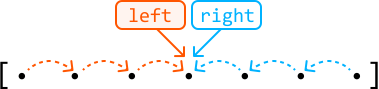
![The image represents a visual depiction of a two-pointer approach to traversing a data structure, likely an array or list. The structure is shown as a sequence of black dots enclosed within square brackets `[ ]`, representing individual elements. An orange rectangle labeled 'left' points a downward arrow to the leftmost element within a subset of the dots. Dashed orange lines with arrowheads connect this element to the next few elements to its right, indicating a traversal from left to right. Similarly, a light-blue rectangle labeled 'right' points a downward arrow to the rightmost element within a different subset of the dots. Dashed light-blue lines with arrowheads connect this element to the preceding few elements to its left, indicating a traversal from right to left. The two pointers, indicated by the orange and light-blue arrows, are moving towards the center of the data structure, suggesting a merging or comparison process commonly used in algorithms like merge sort or two-pointer techniques for finding pairs with a specific sum.](images/img_9955b5622c48.svg)

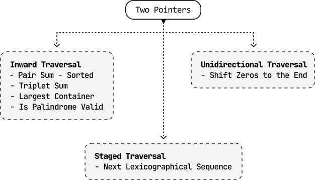
![Image represents a sample input for a coding problem likely related to finding pairs of numbers within an array that sum to a target value. The image shows an integer array `[-5, -2, 3, 4, 6]` enclosed in square brackets, with the index of each element subtly displayed below it (0 through 4). A comma separates the array from the statement 'target = 7,' which specifies the target sum to be found. The arrangement implies that the algorithm should search within the provided array for two numbers that add up to 7. The indices are not explicitly part of the input data but are visually provided to aid understanding of the array's structure.](images/img_4457be769fff.svg)
![Image represents a diagram illustrating a simple summation operation on an array. Two orange rectangular boxes labeled 'left' and 'right' point downwards with arrows towards a numerical array [-5, -2, 3, 4, 6]. The 'left' arrow points to the first two elements of the array, [-5, -2], while the 'right' arrow points to the last three elements, [3, 4, 6]. The array elements are indexed below with numbers 0 through 4, indicating their positions. A separate, light-grey, dashed-line rectangular box displays the result of the summation, showing 'sum = 1'. This implies that the sum of all elements in the array (-5 + -2 + 3 + 4 + 6) equals 1.](images/img_d76971557537.svg)
![Image represents a visual depiction of a two-pointer algorithm, likely used to find a pair of numbers in a sorted array that sum to a target value (not explicitly shown but implied). The top section shows an initial state with two pointers, labeled 'left' and 'right,' pointing to the beginning and end, respectively, of a sorted array [-5, -2, 3, 4, 6]. The indices (0, 1, 2, 3, 4) are shown below the array elements. A dashed box shows the current sum (1, calculated as -5 + 6) being compared to a target value (7, also implied). Since the sum (1) is less than 7, a solid arrow indicates that the 'left' pointer is incremented (left += 1). The bottom section illustrates the updated state after the pointer increment, where the 'left' pointer now points to -2. The 'right' pointer remains unchanged. The dotted arrow emphasizes the movement of the 'left' pointer. The overall diagram demonstrates a single iteration of the algorithm, highlighting the pointer movement based on the comparison of the current sum with the target value.](images/img_a6651bdaea6f.svg)
![Image represents a visual depiction of a coding pattern, likely illustrating a two-pointer approach or a similar algorithm operating on an array. The top section shows an array `[-5, -2, 3, 4, 6]` with pointers labeled 'left' and 'right' initially pointing to the first and last elements respectively. The indices of the array elements are shown below the array. A dashed box displays a condition: `sum = 4 < 7`, indicating that the sum of elements pointed to by 'left' (3) and 'right' (6) is 4, which is less than 7. A thick arrow connects this condition to another dashed box showing the consequence: `left += 1`, signifying that the 'left' pointer is incremented. The bottom section shows the state after this operation: the 'left' pointer has moved one position to the right, now pointing to the element 3, while the 'right' pointer remains unchanged. The 'left' pointer in the bottom section is highlighted in orange to emphasize its movement. The overall diagram illustrates a step-by-step execution of a code segment that iterates through an array, potentially searching for a specific condition or performing a calculation based on the values pointed to by the 'left' and 'right' pointers.](images/img_fdb20ad6f919.svg)
![Image represents a visual depiction of a coding pattern, possibly illustrating a segment of an algorithm. The top section shows an array `[-5, -2, 3, 4, 6]` with indices 0 through 4 labeled below. Above the array, two rectangular boxes labeled 'left' and 'right' point downwards, indicating pointers or indices. The 'left' pointer points to the element '3' (index 2), and the 'right' pointer points to the element '6' (index 4). A dashed box to the right shows a calculation: 'sum = 9 > 7', implying the sum of the elements pointed to by 'left' and 'right' (3 + 6 = 9) is greater than 7. An arrow then points to another box indicating 'right -= 1', suggesting the 'right' pointer's index is decremented. The bottom section shows the updated state after this operation. The array remains the same, but the 'right' pointer (now orange) points to the element '4' (index 3), illustrating the effect of the decrement operation. A dotted line shows the movement of the 'right' pointer from index 4 to index 3. The 'left' pointer remains unchanged.](images/img_d5c13e324a54.svg)
![Image represents a diagram illustrating a coding pattern, possibly related to array processing or a divide-and-conquer algorithm. At the top, two orange rectangular boxes labeled 'left' and 'right' are shown. Arrows descend from these boxes, pointing to the elements '3' and '4' respectively, within a horizontal array represented as `[-5, -2, 3, 4, 6]`. The array indices (0, 1, 2, 3, 4) are displayed beneath the corresponding array elements. A light gray, dashed-bordered rectangle contains the expression 'sum = 7 == 7', indicating a comparison where the sum of some values (implied to be '3' and '4') equals 7. A thick arrow points from this comparison to the text 'return [left, right]', suggesting that if the comparison is true, the function returns an array containing the values 'left' and 'right'. The overall diagram visually depicts the process of selecting elements from an array based on some condition (here, implicitly the sum of selected elements), and returning a result based on those selections.](images/img_49a85e4e420e.svg)
![Image represents a visual depiction of a sorting operation. The image shows an unsorted array `[-1, 2, -2, 1, -1, 2]` enclosed in square brackets on the left. A rightward-pointing arrow labeled 'sort' connects this initial array to a second array `[-2, -1, -1, 1, 2, 2]` also enclosed in square brackets on the right. The arrow indicates the transformation of the input array (on the left) into the sorted output array (on the right) using a sorting algorithm (implied by the label 'sort'). The numbers within each array represent the elements of the array, and their order demonstrates the before-and-after effect of the sorting process. The output array shows the elements of the input array arranged in ascending order.](images/img_96c1f2551d3d.svg)
![Image represents a visual depiction of the `pair_sum_sorted` function's execution on a sorted array `[-2, -1, -1, 1, 2, 2]`, aiming to find triplets summing to a target of 2. The top shows the input array `a` labeled with 'i' indicating an index. An arrow points downwards to the function call `pair_sum_sorted([-1, -1, 1, 2, 2], target = 2)`, excluding the initial -2. The function iteratively uses two pointers, `left` and `right`, initially pointing to the first and last elements of the sub-array, respectively. Each step shows the current array section, the positions of `left` and `right` highlighted in orange boxes, the calculated `sum` of the elements at these positions, and the resulting adjustment to `left` or `right` based on whether the `sum` is less than, greater than, or equal to the target. The process continues until `left` and `right` cross, at which point 'no pairs found' is indicated, implying no triplet starting with -2 sums to 2. Finally, a concluding statement 'no triplet exists that starts with -2' summarizes the function's outcome.](images/img_6ae0b5de32ef.svg)
![Image represents a flowchart illustrating the `pair_sum_sorted` algorithm. The algorithm starts with a sorted input array `[-2, -1, -1, 1, 2, 2]` labeled 'a'. The function `pair_sum_sorted([-1, 1, 2, 2], target = 1)` is then called, indicating a search for pairs summing to 1 within the sub-array `[-1, 1, 2, 2]`. Two pointers, `left` and `right`, initially point to the first and last elements of this sub-array respectively. The algorithm iteratively checks the sum of the elements pointed to by `left` and `right`. If the sum equals the target (1), a pair is found ([-1, 2], labeled 'b' and 'c'), and `left` is incremented to find more pairs. If the sum is greater than the target, `right` is decremented. If the sum is less than the target, `left` is incremented (not explicitly shown but implied). This process continues until `left` and `right` cross, at which point the algorithm terminates. The final result, pairs found `[-1, 2]`, is shown, along with a note indicating how these pairs are added to a result array. The flowchart visually depicts the flow of control and data manipulation within the algorithm, showing the changes in pointer positions and the conditional logic based on the sum of the elements.](images/img_1a17b40cf8c4.svg)

![Image represents two identical examples of a data transformation process. Each example shows a sequence of numbers arranged into three labeled groups: 'a', 'b', and 'c'. Group 'a' contains the numbers [-4, -4, -2, 0], group 'b' contains [0, 1, 2], and group 'c' contains [3]. A rightward arrow indicates a transformation where the first element from each group ('a', 'b', and 'c') – specifically -4, 0, and 3 – are extracted and combined to form a new data structure labeled 'triplet [-4 1 3]'. The arrangement is replicated identically below the first example, emphasizing the consistent application of the transformation rule. The labels 'a', 'b', and 'c' are consistently placed above their respective number groups in both examples.](images/img_dfe398a90541.svg)
![Image represents two examples of extracting a triplet from a larger array. Each example shows a numerical array enclosed in square brackets, containing the elements [-4, -4, -2, 0, 0, 1, 2, 3]. Above each element within the array, labels 'a', 'b', and 'c' are placed to identify sections. In both examples, a sub-array consisting of three elements is highlighted with a cyan-colored box. The first example highlights the elements 0, 0, and 1 (labeled b, b, and c respectively), while the second example highlights the elements 0, 0, and 1 (labeled a, b, and c respectively). A rightward arrow connects each array to the resulting 'triplet,' which is represented as [-2, 0, 2] in both cases. Note that the triplet's values are not directly taken from the highlighted sub-array but rather seem to be a result of some transformation or operation not explicitly shown in the diagram.](images/img_7744c39a1897.svg)

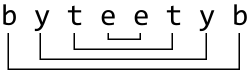
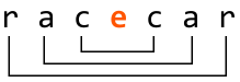
![Image represents a diagram illustrating a coding pattern, possibly related to array or string manipulation. Two orange rectangular boxes labeled 'left' and 'right' are positioned above a line of text 'a + 2 c ! 2 a'. Arrows descend from each box, pointing to the respective ends of this text string. Below, a light-grey, dashed-bordered rectangle contains the conditional statement 's[left] == s[right]', which checks for equality between elements at indices 'left' and 'right' of an array or string 's'. A right-pointing arrow follows this condition, leading to the consequent action 'left += 1, right -= 1', indicating that the 'left' index is incremented and the 'right' index is decremented. The overall diagram suggests an algorithm that iterates through a sequence from both ends, comparing elements until a mismatch is found or the indices cross.](images/img_2d7c0804706c.svg)
![Image represents a diagram illustrating a coding pattern. At the top, two orange rectangular boxes labeled 'left' and 'right' are shown. A downward-pointing arrow extends from each box. Below the boxes, a string 'a + 2 c ! 2 a' is displayed. The 'left' arrow points to the 'a + 2' portion of the string, and the 'right' arrow points to the 'c ! 2 a' portion. A light gray, dashed-bordered rectangle contains the text 's[left] is not alphanumeric → left += 1,' indicating a conditional statement. This statement checks if the character at the index specified by the variable `left` within string `s` is not alphanumeric. If the condition is true, the value of `left` is incremented by 1. The arrow within the gray rectangle visually represents the flow of control based on the condition's outcome.](images/img_873e8234924e.svg)
![Image represents a diagram illustrating a coding pattern, possibly related to string manipulation or array processing. At the top, two orange rectangular boxes labeled 'left' and 'right' are shown. Arrows descend from each box pointing to a string 'a + 2 c ! 2 a'. This string appears to be the input data, with 'left' pointing to the 'a + 2' segment and 'right' pointing to the '2 a' segment. Below the input string, a light gray, dashed-bordered rectangle contains the core logic: 's[left] == s[right] → left += 1, right -= 1'. This expression signifies a comparison: if the element at index 'left' in string 's' is equal to the element at index 'right', then the 'left' index is incremented by 1, and the 'right' index is decremented by 1. This suggests an algorithm that iterates from both ends of the string, comparing elements until a mismatch is found or the indices cross. The arrow ('→') indicates the conditional action taken upon successful comparison.](images/img_50179852d69c.svg)
![Image represents a diagram illustrating a coding pattern, specifically a conditional assignment. At the top, two rectangular boxes labeled 'left' and 'right' (in orange) are shown. Downward arrows from these boxes point to a string 'a + 2 c ! 2 a'. This string appears to represent an input, with 'left' pointing to 'a + 2 c' and 'right' pointing to '! 2 a'. Below this, a light gray, dashed-bordered rectangle contains the conditional statement: 's[right] is not alphanumeric → right -= 1'. This statement indicates that if the substring referenced by `s[right]` (which is '! 2 a' in this example) is not alphanumeric, then the value of the variable `right` is decremented by 1. The arrow ('→') signifies the conditional flow, showing the consequence of the condition being met. The diagram visually demonstrates how the 'right' variable's value might change based on the content of the input string.](images/img_a0a3fdebb003.svg)

![Image represents a diagram illustrating a coding pattern, possibly related to string manipulation or palindrome checking. At the top, two orange rectangular boxes labeled 'left' and 'right' are shown. Arrows point downwards from these boxes to a sequence of characters 'a b b a' below. This sequence appears to be a string being processed. A light gray, dashed-bordered rectangle contains the core logic: 's[left] == s[right] → left += 1, right -= 1'. This expression indicates a comparison: the character at index `left` in string `s` is compared to the character at index `right`. If they are equal (indicated by '=='), then the `left` index is incremented by 1 ('left += 1') and the `right` index is decremented by 1 ('right -= 1'). This suggests an iterative approach, moving inwards from both ends of the string, likely to check for palindromic properties. The arrow ('→') signifies the conditional execution of the index updates based on the comparison result.](images/img_1f92c2cb78df.svg)
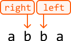
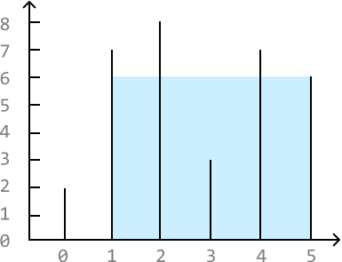
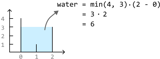
![Image represents a bar chart visualizing the data contained within the Python list `heights = [2, 7, 8, 3, 7, 6]`. The horizontal axis represents the index of each element in the list (0 through 5), while the vertical axis represents the value of each element, ranging from 0 to 8. Each vertical bar corresponds to an element in the list; its height corresponds to the element's value. For example, the first bar at index 0 has a height of 2, the second bar at index 1 has a height of 7, and so on. The vertical axis is marked with numerical labels (0 through 8) indicating the height of the bars, and the horizontal axis is implicitly marked by the position of the bars, corresponding to the list indices. The arrowheads on the axes indicate the direction of increasing values.](images/img_7c18be879c78.svg)
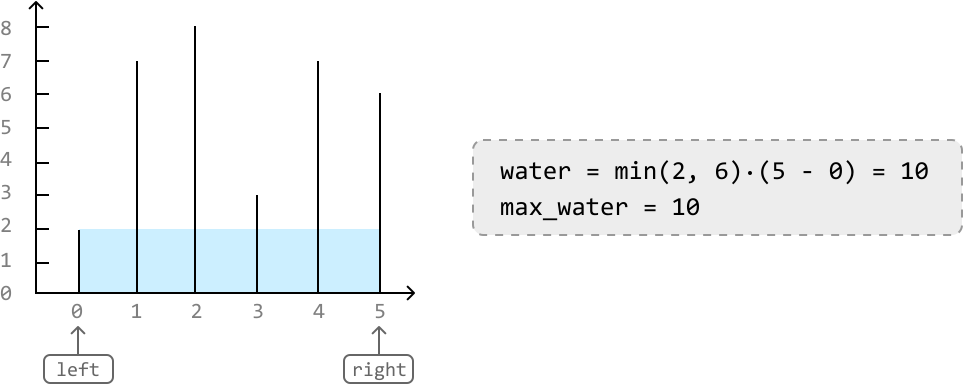
![Image represents a visual explanation of a coding pattern, likely related to algorithms operating on arrays or lists. The left side shows a bar chart with a horizontal axis labeled from 0 to 5 and a vertical axis representing height from 0 to 8. Several bars of varying heights are displayed; the heights are implicitly represented by the vertical extent of the bars. A light-blue rectangle fills the area below the height of the bars, representing a water level. An orange box labeled 'left' points to the leftmost bar, and another orange box labeled 'right' points to the rightmost bar. These labels 'left' and 'right' likely represent index pointers within an array. On the right side, a light-grey dashed-bordered box contains a conditional statement in code-like notation: `heights[left] < heights[right] → left += 1`. This indicates that if the height at the index `left` is less than the height at the index `right`, then the `left` index is incremented by 1. The arrow implies a flow of information or control; the condition's evaluation dictates the update of the `left` pointer. The overall diagram illustrates a step within an algorithm, possibly for finding the largest rectangular area in a histogram or a similar problem involving array traversal and comparison.](images/img_20a1bae7f7bb.svg)
![Image represents a bar chart illustrating a coding pattern, likely related to finding the maximum area of water trapped between vertical bars. The horizontal axis shows indices (0 to 5), and the vertical axis represents heights. Vertical bars of varying heights are drawn at each index; their heights are 2, 6, 6, 3, 6, and 0 respectively. A light-blue area is filled between the bars at indices 1, 2, 3, and 4, representing the trapped water. Arrows labeled 'left' and 'right' point towards the x-axis, indicating the direction of traversal in an algorithm. A separate box contains code snippets: `water = min(7, 6) * (5 - 1) = 24` calculates the water trapped between specific bars (likely using the minimum height as the limiting factor and the distance between them), `max_water = 24` stores the maximum water found so far, and `heights[left] > heights[right] → right -= 1` shows a conditional statement, suggesting an algorithm iterates from left and right, moving the right pointer inwards if the left bar is taller. The overall diagram visually explains a two-pointer approach to solving a 'trapping rain water' problem.](images/img_e4ccba861b43.svg)
![Image represents a bar chart illustrating a 'two-pointer' approach to finding the maximum area that can be contained between vertical bars. The horizontal axis shows indices (0 to 5), and the vertical axis represents height. Several vertical bars of varying heights are depicted; one bar at index 0 has a height of 2, a group of bars from index 1 to 3 have a height of 7, and a bar at index 3 has a height of 6. The area between the bars at indices 1 and 3 is shaded light blue, representing the calculated water trapped between them. Two orange rectangular boxes labeled 'left' and 'right' point to the indices 1 and 4 respectively, indicating the pointers used in the algorithm. A separate box displays calculation details: `water = min(7, 7) * (4 - 1) = 21`, showing the calculation of the water trapped between the pointers; `max_water = 24` indicates the maximum water trapped found so far; and `heights[left] == heights[right] => left += 1 and right -= 1` describes the algorithm's logic: if the heights at the left and right pointers are equal, both pointers move inwards.](images/img_d9ba0d95a1ed.svg)
![Image represents a diagram illustrating a coding pattern, likely related to finding the maximum trapped rainwater between vertical bars. The left side shows a bar chart with vertical bars of varying heights (1, 7, 3, 7, 6) at positions 0, 1, 2, 3, 4, 5 respectively on the x-axis and heights on the y-axis. A light-blue rectangle is filled between bars of height 3 and 7 at positions 2 and 3, representing trapped water. Below the chart, orange rectangular boxes labeled 'left' and 'right' indicate pointers or indices used to iterate through the bars. An arrow points upwards from 'left' to the bar at position 2 and another from 'right' to the bar at position 3. The right side contains a light-grey box with code-like annotations. These annotations show a calculation: `water = min(8, 3) * (3 - 2) = 3`, indicating the calculation of water trapped between two bars; `max_water = 24`, representing the maximum trapped water; and `heights[left] > heights[right] => right -= 1`, suggesting a conditional statement controlling the movement of the 'right' pointer based on the heights of the bars at the 'left' and 'right' indices. The overall diagram visually explains an algorithm for calculating maximum trapped rainwater using two pointers.](images/img_63b24e5abce3.svg)
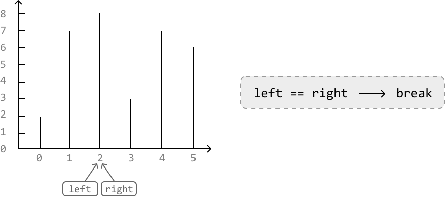
![The image represents a data transformation process. It shows an input array `[0 1 0 2 3]` enclosed in square brackets. A light-blue rectangular box highlights the non-zero elements (1, 2, and 3) within this array. A solid black arrow points from the input array to an output array `[1 2 3 0 0]`. Below the input array, the text 'non-zero numbers go here' in light-blue indicates that the transformation involves extracting only the non-zero numbers. Light-blue horizontal lines are drawn under both the input and output arrays, visually connecting the non-zero elements in the input to their corresponding positions in the output, implying a direct mapping of non-zero values. The zeros in the input array are preserved in the output array, maintaining the original array's length.](images/img_bece262ce41f.svg)
![Image represents a visualization of a coding pattern, likely illustrating pointer manipulation within an array. The top section shows two gray boxes labeled 'left' and 'right' pointing downwards to an array `[0 1 0 2 3]`. This represents the initial state of the array and the pointers. Below, a second similar arrangement shows the array after a step in the algorithm. The 'left' pointer remains unchanged, but the 'right' pointer (shown in orange) has moved one position to the right. A dashed gray box in the middle displays a conditional statement: `nums[right] == 0 → right += 1`, indicating that if the element at the index pointed to by 'right' is equal to 0, then the value of 'right' is incremented. The dashed line connecting the 'right' pointer in the second array to the conditional statement visually connects the conditional check to the pointer's movement. The overall diagram illustrates a single iteration of an algorithm that likely involves traversing and manipulating an array using two pointers.](images/img_f1b4988b01d1.svg)
![Image represents a visual depiction of a sorting algorithm's step. Two rectangular boxes labeled 'left' and 'right' are positioned above a horizontal array `[0 1 0 2 3]`. Arrows descend from 'left' and 'right' pointing to the array elements at indices 0 and 1 respectively. A dashed-line rectangle to the right contains the conditional statement 'nums[right] != 0 → swap(nums[left], nums[right])', indicating that if the element at the index pointed to by 'right' (which is 1 in this case) is not equal to 0, then a swap operation occurs between the elements at the indices pointed to by 'left' and 'right'. The 'nums' refers to the array, and 'left' and 'right' act as index pointers. The arrow '→' signifies the conditional execution of the swap function.](images/img_16ddf7778e6c.svg)
![Image represents a visual depiction of a swap operation within a sorting algorithm, likely a variation of quicksort or similar. At the top, two rectangular boxes labeled 'left' and 'right' are shown, each with a downward-pointing arrow. These arrows point to a numerical array represented as `[1 0 2 3]`, where the numbers 1 and 0 are highlighted in light peach circles. A gray horizontal line connects the numbers 1 and 0, indicating their positions within the array. A curved orange arrow, labeled 'swapped,' arcs underneath the line, connecting the circled 1 and 0, illustrating the exchange of these two elements. The overall diagram demonstrates a single swap step in a sorting process, where the values pointed to by 'left' and 'right' pointers are interchanged.](images/img_7ba7ec46c0b9.svg)
![The image represents a simple illustration of a coding pattern, possibly related to array manipulation or pointer movement. Two rectangular boxes labeled 'left' and 'right' are positioned above a horizontal line segment. Downward arrows connect each box to a number below the line. The numbers below the line are arranged as an array-like structure: `[1 0 0 2 3]`. A dashed-line rectangle to the right contains the text 'left += 1, right += 1', indicating an operation where the values associated with 'left' and 'right' are incremented by 1. The arrows suggest that the 'left' and 'right' variables might represent indices or pointers into the array, and the operation in the dashed box describes how these indices are updated. The overall diagram visually depicts a step in an algorithm that involves iterating or manipulating an array using two pointers.](images/img_cb4f8204d47d.svg)
![Image represents a diagram illustrating a coding pattern, possibly related to array traversal or pointer manipulation. Two rectangular boxes labeled 'left' (in orange) and 'right' (in gray) are positioned at the top. A solid downward-pointing arrow extends from each box, indicating data flow. These arrows point to the numbers 0 and 0 respectively, which are situated below on a horizontal gray line representing an array or sequence. The number 1 is placed to the left of the 0 from the 'left' box, and the number 2 and 3 are placed to the right of the 0 from the 'right' box, all on the same horizontal line, enclosed within square brackets `[ ]` to denote an array structure. A dashed orange arrow connects the 'left' box's output (0) to the number 1, suggesting a possible indirect or conditional relationship or data flow. The overall arrangement suggests a process where the 'left' and 'right' elements might represent pointers or indices that traverse the array, potentially converging or interacting at a central point (the 0s).](images/img_c18f311953b4.svg)
![Image represents a diagram illustrating a coding pattern, possibly within a sorting or searching algorithm. Two rectangular boxes labeled 'left' and 'right' are positioned above a horizontal array represented by `[1 0 0 2 3]`. Arrows descend from 'left' and 'right' pointing to the array elements at indices 1 and 2 respectively (the values 0 and 0). A separate, light-grey, dashed-bordered rectangle to the right contains a conditional statement: `nums[right] == 0 -> right += 1`. This indicates that if the element at the index `right` in the `nums` array is equal to 0, then the value of `right` is incremented by 1. The diagram visually shows the variables `left` and `right` potentially used as pointers or indices within the array, and the conditional statement describes a step in an algorithm that modifies the `right` pointer based on the value of the array element it points to.](images/img_291d5cd7aca2.svg)
![Image represents a simplified illustration of a data structure, possibly an array, being manipulated. Two rectangular boxes, labeled 'left' (in gray) and 'right' (in orange), represent pointers or indices. A gray horizontal line depicts an array containing the elements [1, 0, 0, 2, 3]. A solid downward-pointing arrow from 'left' points to the element '0' at index 1, indicating that the 'left' pointer is currently at this position. An orange downward-pointing arrow from 'right' points to the element '2' at index 3, showing the 'right' pointer's position. A dashed orange curved arrow connects the 'right' pointer to the element '0' at index 2, suggesting a potential movement or operation involving this element. The overall arrangement visualizes the pointers' positions within the array and hints at a possible algorithm or process involving these pointers, perhaps related to partitioning or searching within the data structure.](images/img_d1333351032f.svg)
![Image represents a visual depiction of a step in a sorting algorithm, likely a comparison-based sort. Two rectangular boxes labeled 'left' and 'right' are positioned above a horizontal array `[1, 0, 0, 2, 3]`. Arrows descend from 'left' and 'right' pointing to the array elements at indices 1 and 4 respectively (0 and 2). A dashed-line rectangle to the right displays the condition `nums[right] != 0` followed by a right arrow and the action `swap(nums[left], nums[right])`. This indicates that if the element at the index pointed to by 'right' (which is 2) is not equal to 0, then the elements at the indices pointed to by 'left' and 'right' (0 and 2) will be swapped. The diagram illustrates a single comparison and potential swap operation within a larger sorting process.](images/img_ef9e5627b01a.svg)
![Image represents a visual depiction of a swapping operation within an array. The diagram shows an array `[1, 2, 0, 3]` with two pointers, labeled 'left' and 'right,' initially pointing to the elements 2 and 0 respectively. Arrows from rectangular boxes labeled 'left' and 'right' indicate the pointers' positions. A gray horizontal line connects the elements 1, 2, 0, and 3, representing the array. A curved orange arrow labeled 'swapped' shows the exchange of the values at the 'left' and 'right' pointer positions. To the right, a light gray, dashed-bordered rectangle contains the operation `left += 1, right += 1`, indicating that after the swap, both pointers will increment their positions by one in the next iteration. The overall image illustrates a single step in a sorting algorithm, likely involving a swap and pointer movement.](images/img_be14174bbf44.svg)
![Image represents a diagram illustrating a simple coding pattern, possibly related to array manipulation or pointer movement. The diagram shows a numerical array `[1 2 0 0 3]` represented horizontally. Above the array, two rectangular boxes labeled 'left' and 'right' in orange are positioned. A solid orange arrow descends from 'left' pointing to the element '0' in the second position from the left within the array. Similarly, a solid orange arrow descends from 'right' pointing to the element '3' at the right end of the array. Dashed orange lines curve from 'left' to the element '2' and from 'right' to the element '0' in the third position, suggesting a potential search or traversal pattern. The overall arrangement suggests a process where two pointers, one starting from the left and the other from the right, might be moving towards the center of the array, potentially for comparison, searching, or merging operations.](images/img_9e4dbe0ba394.svg)
![Image represents a visual depiction of a step in a sorting algorithm, likely a part of a larger process. Two rectangular boxes labeled 'left' and 'right' are positioned above a numerical array `[1, 2, 0, 0, 3]`. Arrows descend from 'left' and 'right' pointing to the '0' elements within the array, indicating these are the current indices being considered. A dashed-line rectangle to the right shows a conditional statement: `nums[right] != 0 → swap(nums[left], nums[right])`. This indicates that if the element at the index 'right' is not equal to 0, then a `swap` function is called to exchange the values at the 'left' and 'right' indices within the `nums` array. The arrow represents the flow of control based on the condition.](images/img_5978c4fe5e3c.svg)
![Image represents a visual depiction of a swapping operation within an array. The diagram shows an array `[1, 2, 3, 0]` with two pointers, 'left' and 'right', initially pointing to the elements 3 and 0 respectively. Rectangular boxes labeled 'left' and 'right' above indicate the pointers' origins. A downward-pointing arrow from each box connects to its corresponding element in the array. The elements 3 and 0 are highlighted in light peach. A gray horizontal line connects the elements 1 and 2, visually representing the array's structure. A curved orange arrow labeled 'swapped' connects the highlighted elements 3 and 0, indicating that these elements have been exchanged. To the right, a light gray, dashed-bordered rectangle displays the operation performed: `→ left += 1, right += 1`, signifying that after the swap, both pointers will increment their positions by one.](images/img_909bade58ac3.svg)
![Image represents a diagram illustrating a coding pattern, possibly related to array manipulation or pointer movement. The diagram shows a light-blue rectangular array `[1 2 3]` with a light-blue underline indicating its boundaries. Two orange rectangular boxes labeled 'left' and 'right' are positioned above the array. Dashed orange arrows point downwards from 'left' and 'right' to the array elements. The 'left' arrow points to the first element (1) and the 'right' arrow points to the last element (3). The arrows suggest that the 'left' and 'right' variables might represent pointers or indices that can be manipulated to traverse the array. The empty space `∅` between the array and the pointers suggests an initial state or a potential intermediate step in an algorithm. The overall structure suggests a two-pointer approach commonly used in algorithms like merging or partitioning.](images/img_0913b36a8764.svg)
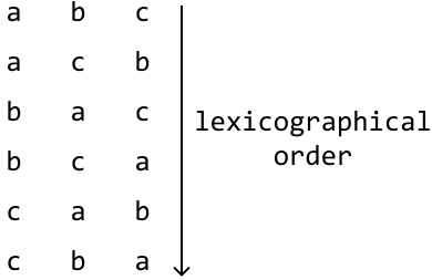
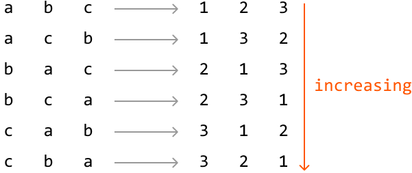
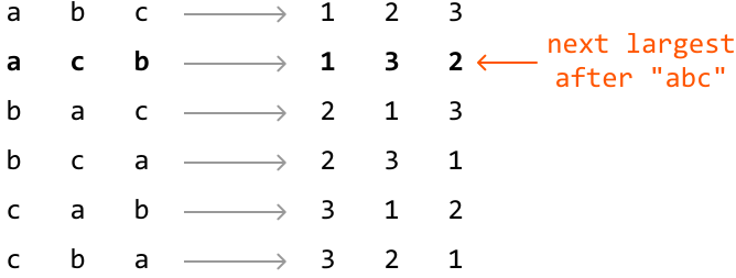
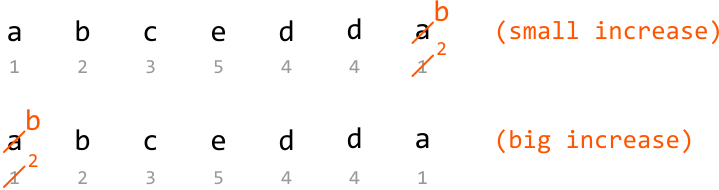

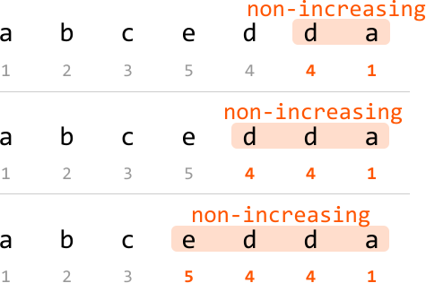

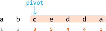

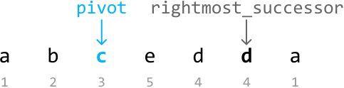



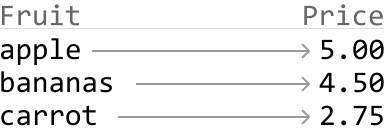
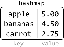
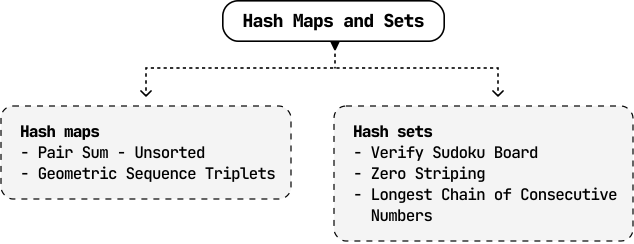
![Image represents a transformation of a numerical array into a hashmap. The input is an array `[-1, 3, 4, 2]` with indices `[0, 1, 2, 3]` displayed beneath each element. A rightward arrow indicates the transformation process. The output is a hashmap labeled 'hashmap' which is represented as a table with two columns: 'num' and 'index'. The 'num' column lists the numbers from the input array: -1, 3, 4, and 2. The corresponding 'index' column shows the original index of each number in the input array: 0, 1, 2, and 3 respectively. The diagram illustrates how the original array's elements and their indices are reorganized into a key-value pair structure within the hashmap, where the number acts as the key and its original index acts as the value.](images/img_e13658bc639a.svg)
![Image represents a sample input for a search algorithm, likely a target-sum problem. The input consists of a numerical array [-1, 3, 4, 2] enclosed in square brackets, with each element implicitly indexed from 0 to 3 shown in grey below the array. This array is separated by a comma from the target value, which is explicitly stated as 'target = 3'. The arrangement suggests the algorithm's task is to find a subset of numbers within the array that sums up to the target value of 3. There is no explicit flow of information depicted; the image simply presents the input data for the algorithm to process.](images/img_5262caac86bc.svg)
![Image represents a data flow diagram illustrating a step in a coding pattern, likely involving hashmaps. An input array `[-1, 3, 4, 2]` with indices [0, 1, 2, 3] is shown. An orange arrow labeled 'x' points to the first element, -1. This array flows into a rectangular box labeled 'hashmap' with internal labels 'num' and 'index' suggesting it stores key-value pairs. To the right of the hashmap is a dashed-line box detailing the processing steps: first, it checks if the hashmap contains -1 (it doesn't); second, it calculates the complement of 4 (presumably within the context of the algorithm); and third, it adds the key-value pair (-1, 0) to the hashmap. The diagram visually depicts the input array, its processing through a hashmap, and the specific operations performed on the hashmap based on the input.](images/img_ffd2c92bfb2a.svg)
![Image represents a step-by-step illustration of a coding pattern involving a hashmap. An input array `[-1, 3, 4, 2]` is shown, with a small orange arrow pointing downwards to the element '3' at index 1, indicating the current element being processed. This array is then processed, resulting in a hashmap represented as a table with two columns labeled 'num' and 'index'. Currently, the hashmap contains only one entry: -1 at index 0. To the right of the hashmap is a dashed-line box containing three bullet points describing the processing logic: '- hashmap doesn't contain 3's', indicating that the current element (3) is not yet in the hashmap; 'complement (0)', suggesting a calculation of the complement (likely 0 in this context); and '- add (3, 1) to hashmap', indicating that the pair (3, 1) – the element and its index – will be added to the hashmap as the next step. The arrow between the array and the hashmap shows the data flow from the input array to the hashmap during processing.](images/img_33cf4992bc46.svg)
![Image represents a data transformation process. An input array `[-1, 3, 4, 2]` with indices [0, 1, 2, 3] is shown. A downward-pointing orange arrow labeled 'x' highlights the element '4' at index 2. This array is then transformed into a hashmap labeled 'hashmap' which has two key-value pairs. The key 'num' stores the number -1, and its corresponding value under the 'index' key is 3. The second key-value pair has 'num' as 0 and 'index' as 1. A separate dashed-line box describes the hashmap's content, stating that it 'contains 4's complement (-1)'. The arrow indicates the input array is processed to generate the hashmap, implying a mapping or counting operation where the complement of a number (in this case, 4's complement -1) and its index are stored.](images/img_f89c216ee5f0.svg)
![Image represents a visual depiction of a coding pattern, likely for finding pairs in an array that sum to a target value (here, implicitly zero). The input is an array `[-1, 3, 4, 2]` with indices `0, 1, 2, 3` respectively, shown above a downward-pointing orange arrow labeled 'x', suggesting a target value or operation. This array is processed, with the element '4' (at index 2) highlighted in light green. A rightward arrow indicates the transformation of this array into a hashmap. The hashmap is represented as a box divided into two columns labeled 'num' and 'index'. The 'num' column contains the unique numbers from the input array (-1 and 3), while the 'index' column shows their corresponding indices (0 and 1 respectively). A curved grey arrow connects the highlighted '4' in the input array to the hashmap, implying that the algorithm uses the hashmap to store and retrieve information. Finally, another curved grey arrow originates from the hashmap's 'index' column and points to `[0, 2]` labeled 'return', indicating that the algorithm returns the indices 0 and 2 as the solution, likely because -1 + 4 = 3 (or a similar logic involving the target value). The overall diagram illustrates the use of a hashmap to efficiently find pairs with a specific sum within an array.](images/img_c8da2b89b371.svg)
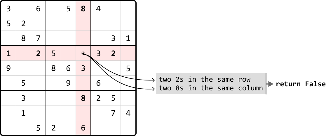
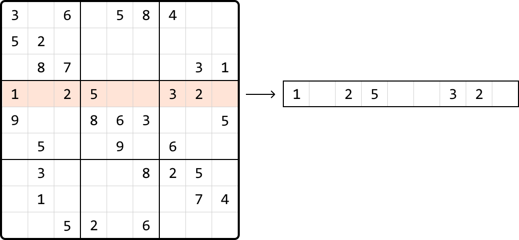





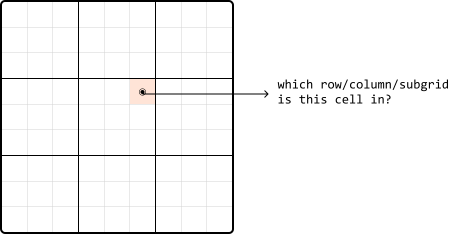

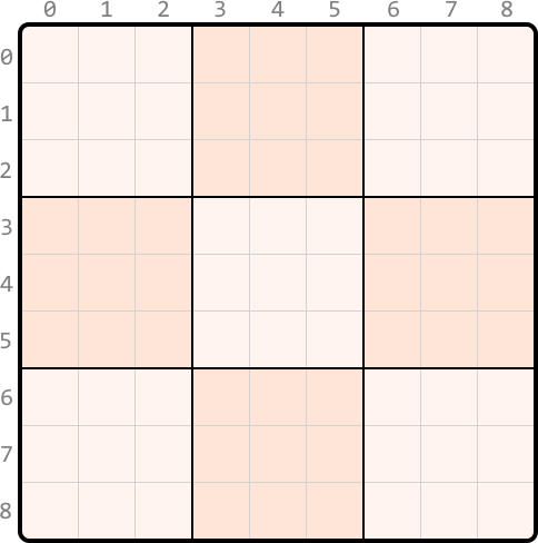
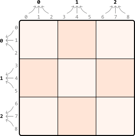
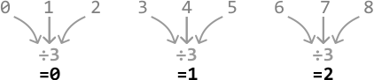
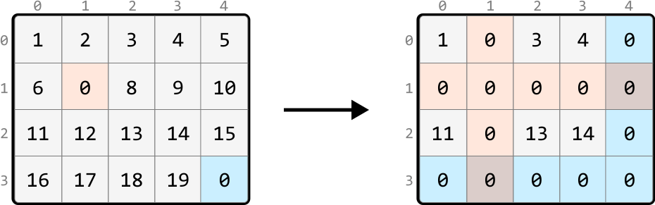
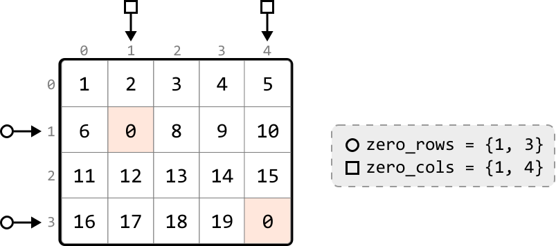
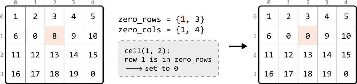
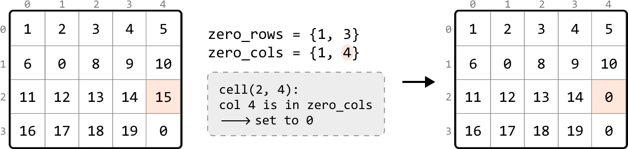
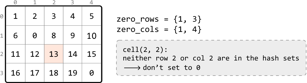
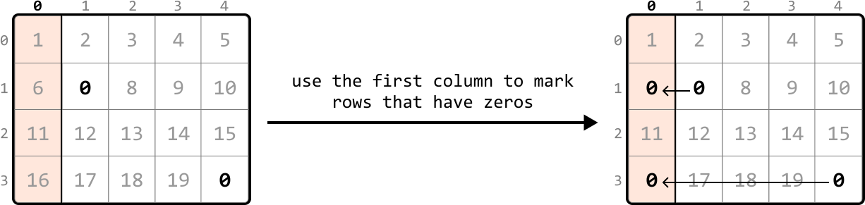
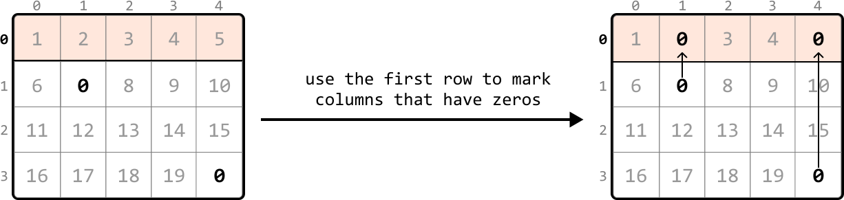
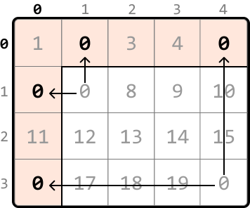
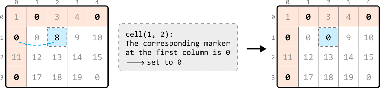
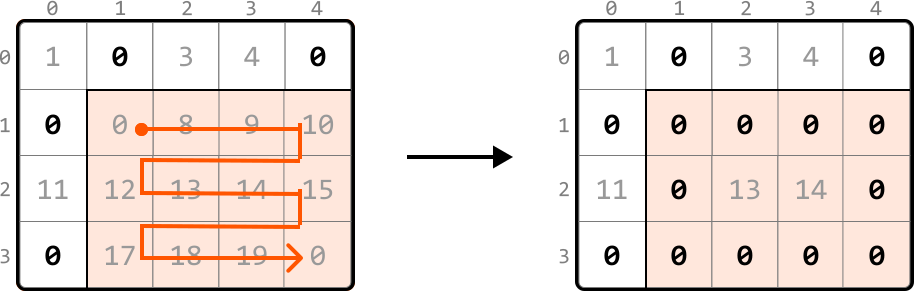
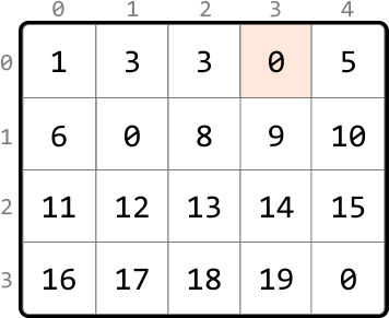
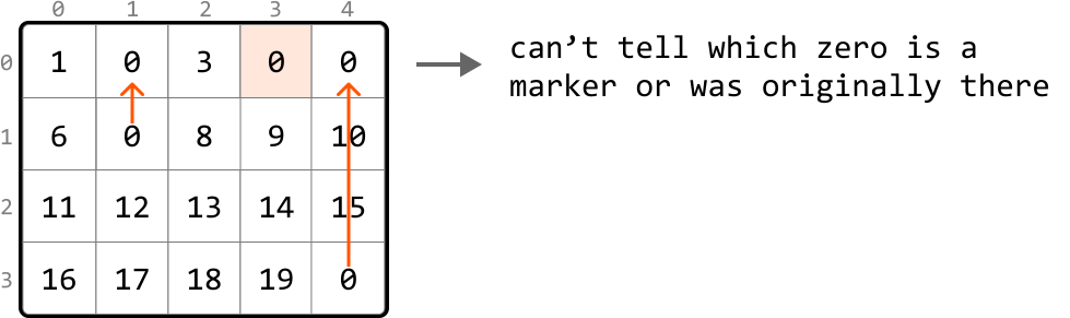
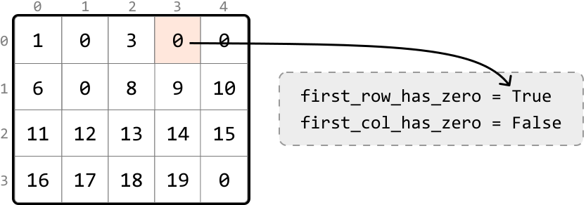
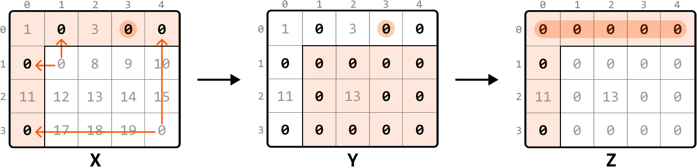
![Image represents a visual depiction of a sorting algorithm's effect on an array of numbers. The diagram begins with an unsorted array `[1 6 2 5 8 7 10 3]` enclosed in square brackets. A right-pointing arrow labeled 'sort' indicates a transformation. The result of the sorting operation is shown as two sub-arrays. The first, a peach-colored sub-array `[1 2 3]`, contains the smallest three numbers from the original array. The second, a light-green sub-array `[5 6 7 8 10]`, contains the remaining numbers, which are larger than those in the first sub-array. The label 'longest' is placed above the second sub-array, indicating that this sub-array represents the longest increasing subsequence within the original unsorted array. The entire output is presented as a sequence of numbers within square brackets.](images/img_d3def0fa08f2.svg)
![Image represents a diagram illustrating a search for a consecutive chain of numbers. The top of the diagram contains the text 'find the rest of a consecutive chain starting at:'. From this text, eight orange arrows point downwards to a set of single-digit numbers enclosed in square brackets: [1, 6, 2, 5, 8, 7, 10, 3]. The arrows visually represent the exploration of potential consecutive chains starting from an unspecified initial number (implied by the phrase 'starting at:'). The numbers at the bottom are potential candidates or elements within the search space for completing the consecutive chain. The diagram suggests a branching or fan-out search strategy, where multiple possibilities are explored simultaneously to find the rest of the consecutive chain.](images/img_8f74615773c5.svg)
![Image represents a diagram illustrating the concept of finding a consecutive chain within a sequence of numbers. The top of the diagram displays the text 'find the rest of a consecutive chain starting at:'. Three orange arrows emanate downwards from this text, pointing to three distinct subsequences of numbers: '[1 6 2]', '[5 8 7]', and '[10 3]'. Below each subsequence, grey arrows indicate potential consecutive chains. Specifically, under '[1 6 2]', a grey arrow points to '1 2 3', suggesting a possible consecutive chain starting with 1. Similarly, under '[5 8 7]', a grey arrow points to '5 6 7 8', indicating a potential consecutive chain starting with 5. Finally, under '[10 3]', a grey arrow points to '10', showing a single-element consecutive chain starting at 10. The diagram visually represents the challenge of identifying consecutive number sequences from a larger, unordered set.](images/img_b8115e057745.svg)
![Image represents a step-by-step illustration of an algorithm, likely searching within an array. The top section shows an array `[1, 6, 2, 5, 8, 7, 10, 3]`. The number 5 is highlighted in a grey circle. Above it, text states 'not the smallest in its chain: 6 - 1 = 5 exists,' indicating a check for whether 5 is the smallest element in a sub-array derived by subtracting 1 from a larger element (in this case, 6). A downward-pointing arrow connects this text to the array, visually indicating the element being processed. The bottom section shows the same array, but now the number 5 is no longer highlighted. Above it, the text reads 'smallest in its chain: 5 - 1 = 4 doesn't exist,' implying that a search for 4 (5-1) within the array failed. A downward-pointing arrow again connects the text to the array, showing that the algorithm continues its search after finding that 5 is not the smallest in its chain. The overall image demonstrates a process of iterating through an array and checking for the existence of specific values derived from calculations on other array elements.](images/img_8f151e96e175.svg)
![Image represents five rows demonstrating a geometric sequence. Each row begins with a bracketed sequence of numbers: [2, 1, 2, 4, 8], with some rows having additional numbers (8) at the end. The numbers 2, 4, and 8 within the brackets are highlighted in peach-colored circles, and small numbers beneath them indicate their position within the sequence (0, 2, 3, 4, 5). Following each bracketed sequence is a colon and then an equation demonstrating the pattern: (2, 2*2 = 4, 4*2 = 8). The first number in the equation (2) corresponds to the first highlighted number in the bracket, and subsequent numbers are generated by multiplying the preceding number by 2. The last row shows a variation where the sequence starts with 1 instead of 2, resulting in a modified equation: (1, 1*2 = 2, 2*2 = 4). The overall image illustrates the concept of a geometric progression where each term is obtained by multiplying the previous term by a constant value (in this case, 2).](images/img_72338d22e002.svg)
![Image represents a diagram illustrating an ordering problem in a data structure. A single 'X' at the top points downwards via a grey arrow to a horizontal array-like structure enclosed in square brackets `[ ]`. This array contains several elements represented by dots (`.`) as placeholders, with a single 'X' and then 'x*r²' and 'x*r' appearing in the array. Below the array, a grey box highlights the text '(x, x*r², x*r)' labeled as 'triplet valves,' indicating that these three elements are expected to form a triplet. The text 'appear in the wrong order' explains that the order of these elements within the array does not match the expected order defined in the triplet valves. The diagram visually shows the incorrect arrangement of the triplet within a larger data structure, highlighting the problem of out-of-order elements.](images/img_b2876bb8e4a0.svg)

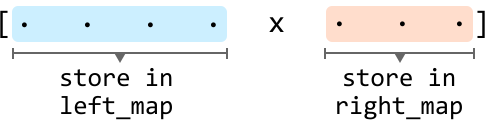
![Image represents a diagram illustrating a coding pattern, possibly related to data structures or algorithms. The diagram shows two parallel structures, each representing a set of numbers. The left structure, labeled 'x/r = 2' in light blue, depicts a set [2, 1, 2], where two instances of the number 2 are connected by a line labeled 'two 2's' to a central node. The right structure, labeled 'x/r = 8' in orange, shows a set [8, 8], with two instances of 8 connected by a line labeled 'two 8's' to the same central node. A downward-pointing arrow labeled 'x' connects the two structures, indicating a transformation or operation. The central node, connected to both structures, is labeled '2 * 2 = 4', suggesting a calculation based on the number of instances in each structure. Finally, an arrow pointing to the right indicates the result: '4 instances of [2, 4, 8]', implying that the combined result of the operation on the two input structures produces four instances of the combined set [2, 4, 8].](images/img_0c85f8335d49.svg)
![Image represents a flowchart illustrating a coding pattern for counting triplets. The top shows two arrays, a light-blue array labeled `[`...`]` on the left representing values of `x/r`, and a peach-colored array labeled `[`...`]` on the right representing values of `x*r`, separated by the variable 'x'. Step ①, labeled 'check that x%r == 0', indicates a condition that must be met. Step ②, labeled 'get frequency of x/r from left_map', shows an arrow pointing from the left array to step ④. Similarly, step ③, labeled 'get frequency of x*r from right_map', shows an arrow pointing from the right array to step ④. Step ④, labeled 'multiply the frequencies to get the number of triplets with this x in the middle', indicates that the frequencies obtained in steps ② and ③ are multiplied to determine the count of triplets where 'x' is the central element, satisfying the condition in step ①. The arrows visually represent the data flow, showing how the frequencies from the left and right arrays are combined to calculate the final result.](images/img_14bf12ee3919.svg)
![Image represents a one-dimensional array or list enclosed in square brackets `[` and `]`, containing the integer sequence `[2, 1, 2, 4, 8, 8]`. This array is separated by a comma from the assignment `r = 2`, indicating a variable `r` is assigned the integer value 2. The arrangement shows the array as a data structure, and the assignment suggests a potential relationship between the array and the variable `r`, possibly representing a parameter or index related to the array's processing or manipulation within a larger algorithm or code. There are no URLs or other parameters present beyond the numerical values and variable assignment.](images/img_9b330384e124.svg)
![Image represents a visual depiction of a data transformation process, likely related to frequency counting or mapping. The input is a list of numbers `[2, 1, 2, 4, 8, 8]` and a value `r = 2`. This input is processed to generate two maps: `left_map` and `right_map`. `right_map` is a table with two columns: `x*r` and `freq`. It shows the results of multiplying each element in the input list by `r` (2) in the `x*r` column, and the frequency of each resulting value in the `freq` column. For example, 2*2=4 appears once, 1*2=2 appears twice, 4*2=8 appears twice. `left_map` is an empty table with columns `x/r` and `freq`, suggesting it would contain the results of dividing each input element by `r` and their corresponding frequencies, but these values are not shown in the image. The overall diagram illustrates a process where an input list is transformed based on a given value `r`, resulting in frequency counts displayed in two separate tables representing different operations (multiplication and division by `r`).](images/img_eb99e69bb40e.svg)
![Image represents a diagram illustrating a coding pattern, possibly related to frequency counting or mapping. The diagram shows an input array `x = [2, 1, 2, 4, 8, 8]` and a value `r = 2`. This input is processed to create two maps: `left_map` and `right_map`. `left_map` is empty, suggesting it's a placeholder or the result of a computation not yet shown. `right_map` is a table with two columns: `x*r` (representing elements of the input array multiplied by `r`) and `freq` (representing the frequency of each element in `x*r`). The `right_map` contains the following entries: `x*r` values of 2, 1, 4, 8 and their corresponding frequencies in `freq` as 2, 1, 1, 2 respectively. An arrow points from the `freq` column value of 2 (corresponding to `x*r` = 2) to the number 1, indicating a potential further processing step or mapping not fully depicted. The overall structure suggests a process where an input array is manipulated based on a given value `r`, resulting in frequency counts displayed in the `right_map`, with a possible additional transformation indicated by the arrow.](images/img_8cc8d6a1fab8.svg)
![The image represents a code snippet illustrating a calculation process. On the left, an array `[2 1 2 4 8 8]` is shown, with a variable `r` assigned the value 2. A downward-pointing arrow suggests this array is input to the process. On the right, a light-grey box contains a conditional statement and a series of calculations. The condition `x % r == 0` checks if a variable `x` (not explicitly defined in the image but implied to be an element from the input array) is divisible by `r`. If true, the `count` variable is updated. The update involves multiplying values from two maps, `left_map` and `right_map`, using `x/r` and `x*r` as indices respectively. The example shows the calculation for `x=2`, resulting in `count += left_map[2/2] * right_map[2*2]`, which simplifies to `count += left_map[1] * right_map[4]`. Subsequent lines show further additions to `count`, ultimately resulting in `count += 0`, suggesting that the initial multiplication resulted in zero, and subsequent additions also contributed zero. The overall structure depicts a conditional update of a counter based on array elements and lookups in two maps (`left_map` and `right_map`).](images/img_1058631b49e7.svg)
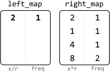
![Image represents a diagram illustrating a coding pattern, possibly related to data processing or algorithm design. At the top, an input array `[2 1 2 4 8 8]` and a parameter `r = 2` are shown. A downward-pointing arrow indicates the processing of the input array. Below, two tables are presented side-by-side, labeled 'left_map' and 'right_map'. 'left_map' contains a column labeled 'x/r' with values (presumably resulting from dividing elements of the input array by `r`) and a column labeled 'freq' representing their frequencies. Similarly, 'right_map' has columns 'x*r' (likely representing multiplication of input array elements by `r`) and 'freq' showing their frequencies. A light gray rectangular box displays the condition `x % r != 0 → can't form a triplet → continue`, indicating that if the remainder of an element divided by `r` is not zero, a triplet cannot be formed, and the process continues to the next element. The overall diagram suggests a frequency analysis or counting process involving division and multiplication by a given parameter `r`, with a conditional check for triplet formation.](images/img_a5bf5c907cdf.svg)
![Image represents a diagram illustrating a coding pattern, possibly related to frequency counting or data manipulation. At the top, an input array `[2 1 2 4 8 8]` and a value `r = 2` are given. Below, two tables labeled 'left_map' and 'right_map' are shown. 'left_map' contains two columns: 'x/r' representing values after integer division by `r`, and 'freq' representing their frequencies. Similarly, 'right_map' has columns 'x*r' (values after multiplication by `r`) and 'freq'. The values in these tables seem pre-calculated based on the input array. A dashed-line box to the right shows a calculation process. It starts with a condition `x % r == 0`, implying a check for divisibility by `r`. If true, a `count` variable is updated by adding the product of a value from 'left_map' (indexed by `x/r`) and a value from 'right_map' (indexed by `x*r`). An example calculation is shown, where `x` is implicitly 2, resulting in `left_map[2/2] * right_map[2*2]`, which simplifies to `1 * 1`, adding 1 to the `count`. The entire process suggests an algorithm that uses pre-computed frequency maps ('left_map' and 'right_map') to efficiently process the input array based on divisibility by `r`.](images/img_da18904f20a3.svg)
![Image represents a diagram illustrating a coding pattern, possibly related to frequency counting or data manipulation. At the top, an input array `[2 1 2 4 8 8]` and a value `r = 2` are given. Below, two tables labeled 'left_map' and 'right_map' are shown. 'left_map' has two columns: 'x/r' (representing the element of the input array divided by r) and 'freq' (frequency). It contains the values 2 (x/r) and 2 (freq) in the first row, and 1 (x/r) and 1 (freq) in the second row. 'right_map' similarly has columns 'x*r' (element multiplied by r) and 'freq', with values 2 and 0, 1 and 0, 4 and 0, and 8 and 2. To the right, a dashed box shows a calculation: `x % r == 0 → count += left_map[x/r] * right_map[x*r]`. This formula is then broken down step-by-step, substituting values from the input array and the maps: `+= left_map[4/2] * right_map[4*2]`, `+= 2 * 2`, and finally `+= 4`, demonstrating how the count is updated based on the values in the 'left_map' and 'right_map' tables. The overall diagram visualizes a process where an input array is processed using two pre-computed frequency maps ('left_map' and 'right_map') to calculate a final count.](images/img_b59d99b4bcc2.svg)
![Image represents a coding pattern illustration focusing on a calculation involving two maps, `left_map` and `right_map`, and an input array `[2, 1, 2, 4, 8, 8]` with `r` set to 2. An arrow points downwards from 'x' suggesting an input value. `left_map` and `right_map` are presented as tables with two columns: the first labeled 'x/r' or 'x*r' respectively, representing the result of integer division by `r` or multiplication by `r`, and the second labeled 'freq', likely representing frequency counts. The `left_map` contains entries (2,2), (1,1), (4,1), (8,1), while `right_map` contains (2,0), (1,0), (4,0), (8,1). A dashed box to the right shows a calculation process: `x % r == 0` (checking if `x` is a multiple of `r`) leads to `count += left_map[x/r] * right_map[x*r]`. The calculation is further broken down with example values, showing `count` being updated by adding the product of `left_map[8/2]` (which is 1) and `right_map[8*2]` (which is 1), resulting in a final `count` of 0. The diagram illustrates how the maps are used to perform a calculation based on the input array and the value of `r`.](images/img_04839d1006fb.svg)
![Image represents a diagram illustrating a coding pattern, possibly for counting occurrences based on modulo operation. At the top, an input array `[2 1 2 4 8 8]` and a value `r = 2` are given. Below, two tables labeled 'left_map' and 'right_map' are shown side-by-side. Each table has two columns: the first column in 'left_map' lists the elements of the input array divided by `r` (integer division), while the second column represents their frequencies. Similarly, 'right_map' has its first column listing elements of the input array multiplied by `r`, and the second column showing their frequencies. A dashed-line box to the right contains a calculation sequence. It starts with a condition `x % r == 0`, indicating that if an element `x` modulo `r` equals 0, a counter (`count`) is updated. The update involves multiplying the frequency from 'left_map' (using the integer division of `x` by `r` as the index) with the frequency from 'right_map' (using `x` multiplied by `r` as the index). The example calculation shows how this is done for the element 8: `left_map[8/2]` (which is 1) is multiplied by `right_map[8*2]` (which is 0), resulting in 0 being added to the counter. The final result of the calculation is 0 in this specific example.](images/img_4a46e5e59ca1.svg)
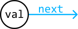


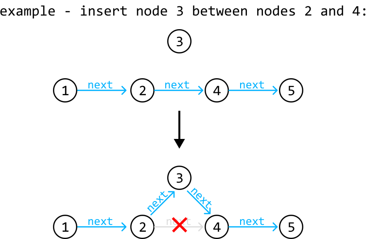

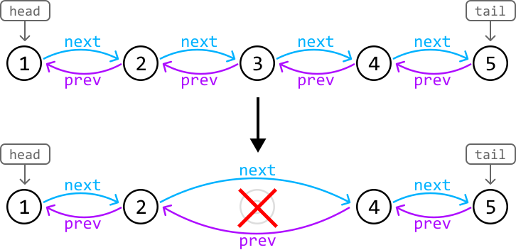
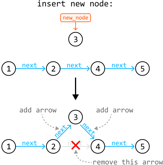
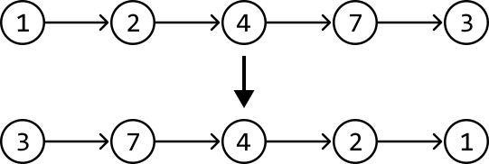
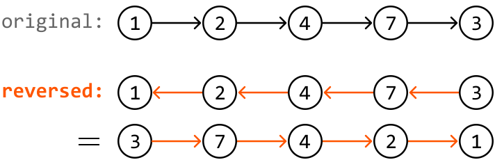


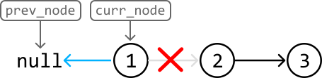
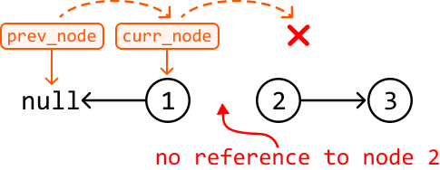

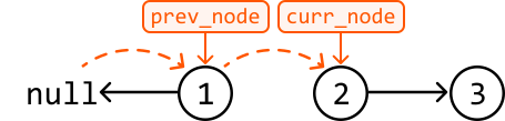

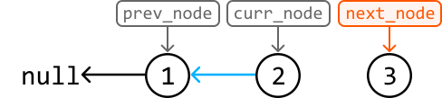

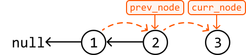




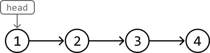




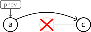

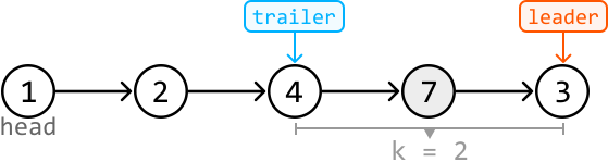

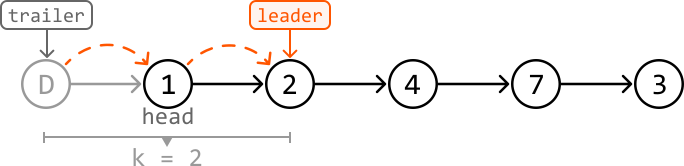





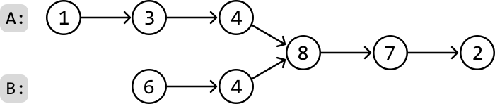
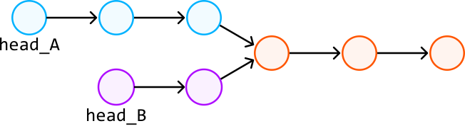
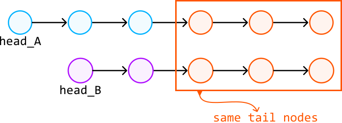
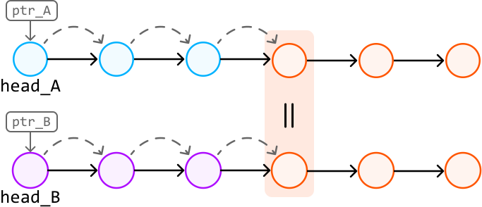
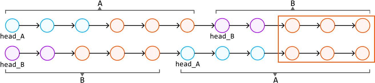
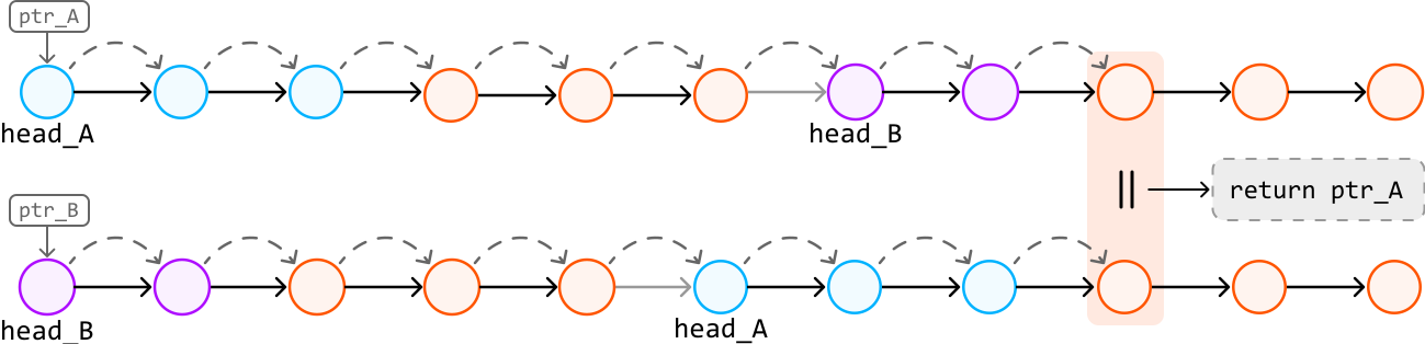
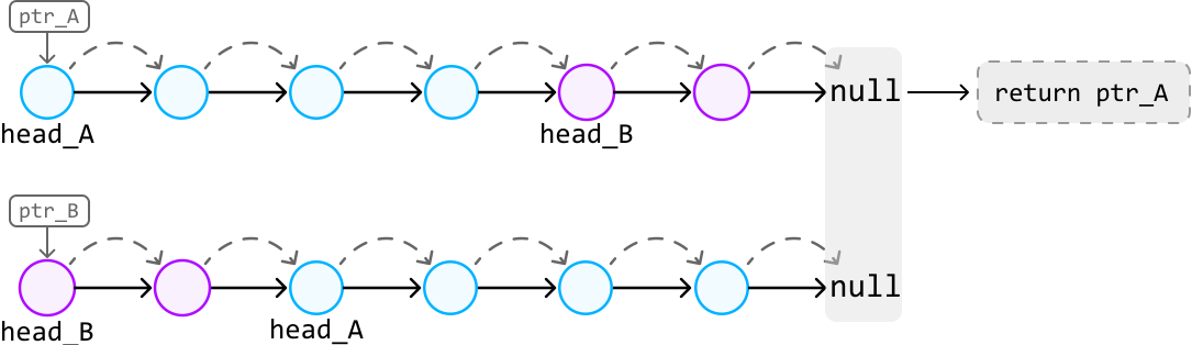
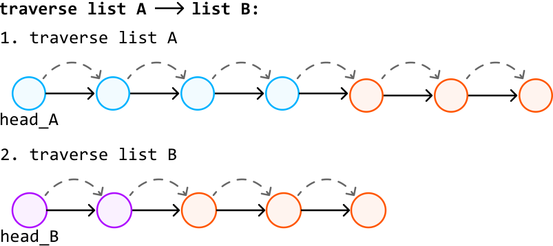
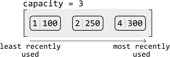
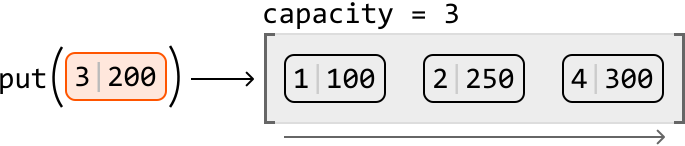
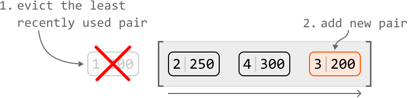
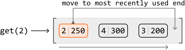



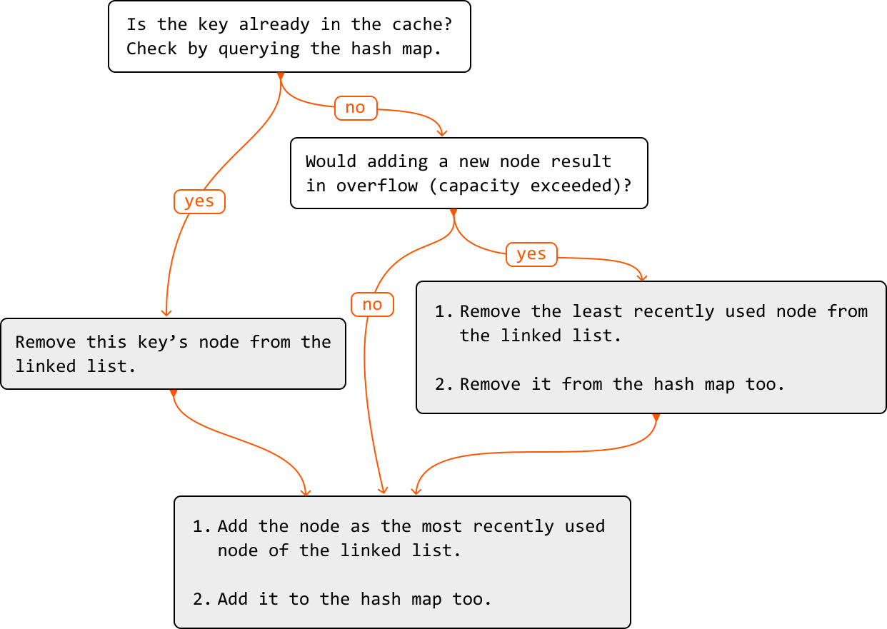
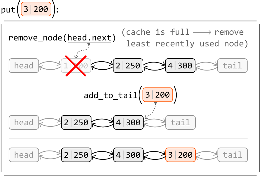
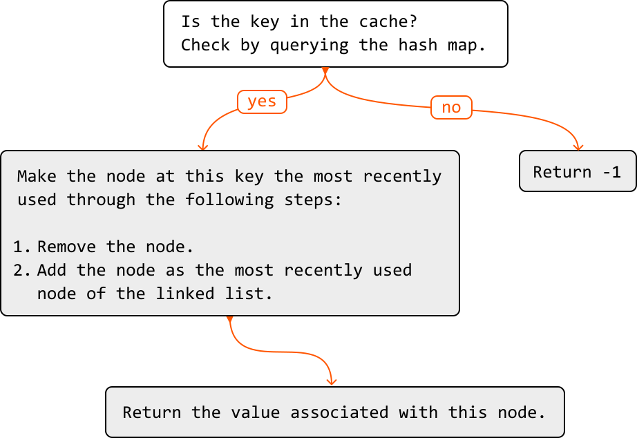
![Image represents a visual depiction of a `get(2)` operation on a doubly linked list, implemented using a hashmap for efficient node access. The top section shows the initial state: a doubly linked list with nodes labeled '2 | 250', '4 | 300', and '3 | 200', connected by bidirectional arrows indicating `next` and `prev` pointers. 'head' and 'tail' labels point to the beginning and end of the list, respectively. A dashed arrow points from `remove_node(hashmap[2])` to node '2 | 250', which is marked with a red 'X', signifying its removal. The middle section illustrates the removal of node '2 | 250'. The bottom section shows the node '2 | 250' re-added to the tail of the list via `add_to_tail(2 | 250)`, indicated by a dashed arrow. Finally, a thick black arrow at the bottom points to 'return 250', indicating the value returned by the `get(2)` operation after the node has been temporarily removed and then re-added to the tail. Each node displays a key-value pair (e.g., '2 | 250'), representing the key used in the hashmap and the associated value. The overall diagram demonstrates the process of retrieving a node's value, removing it, and then re-inserting it at the tail to maintain the list's structure.](images/img_6e3ecbd72e54.svg)
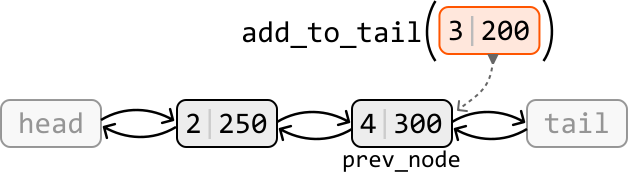
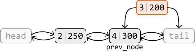



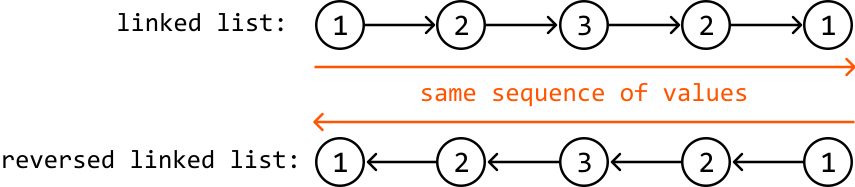
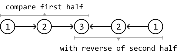
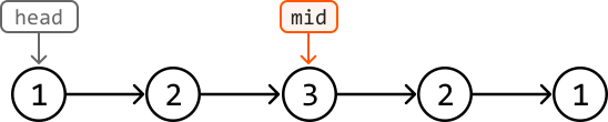

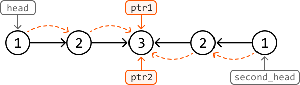
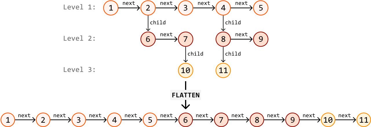
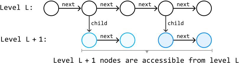
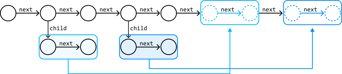
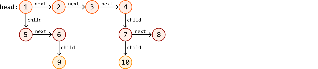

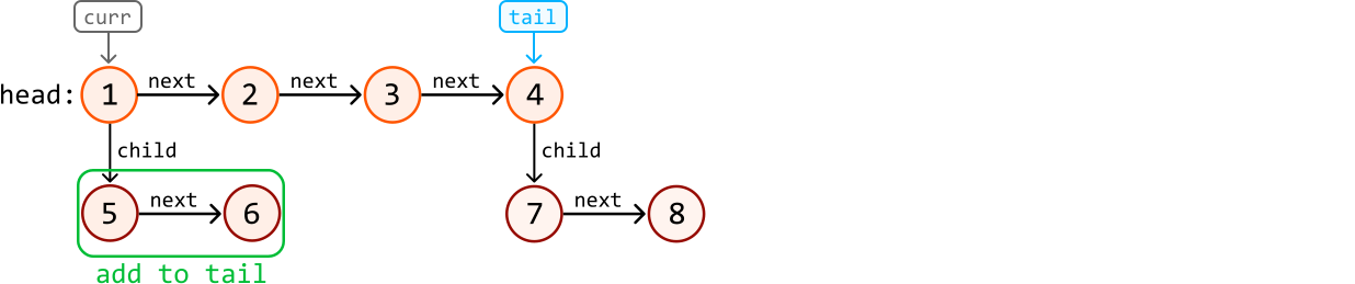



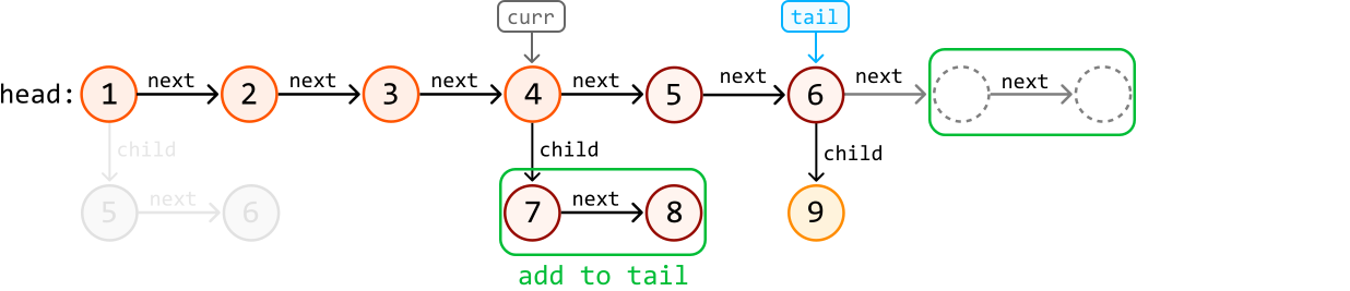
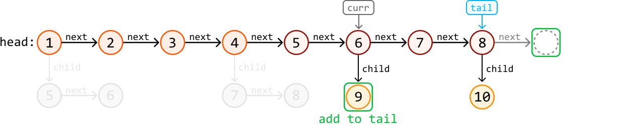


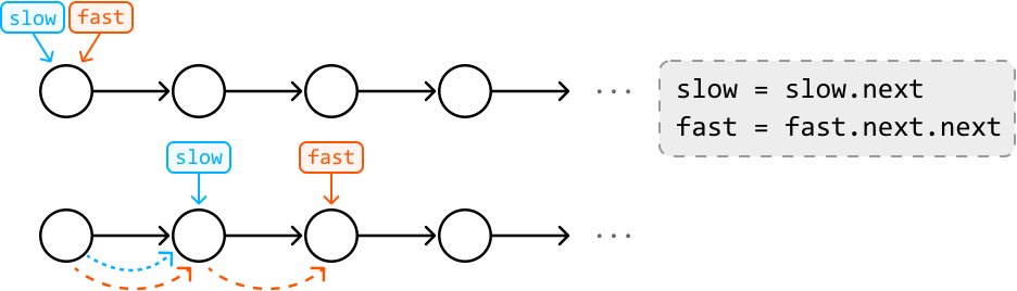
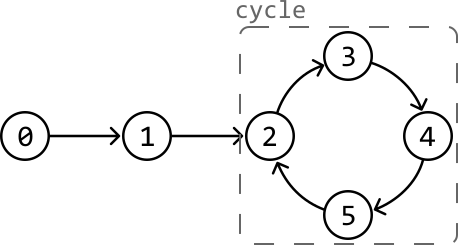
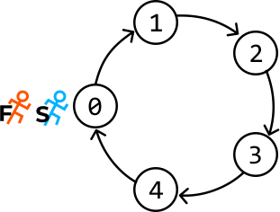
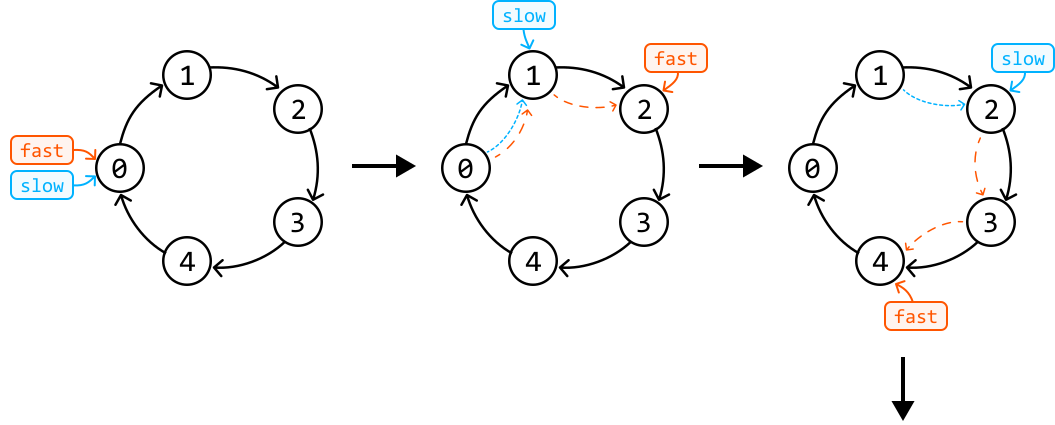
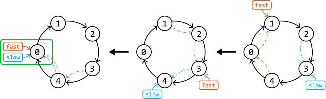
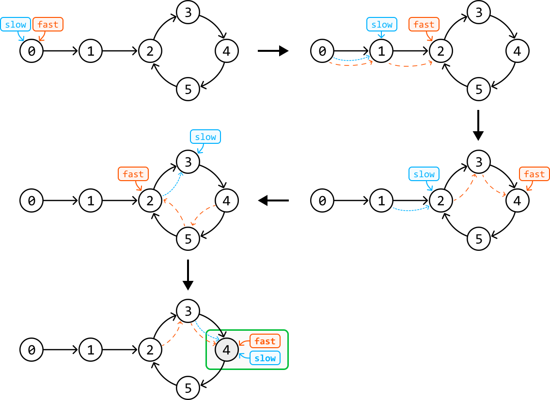
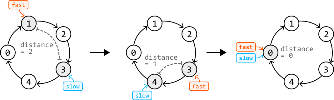



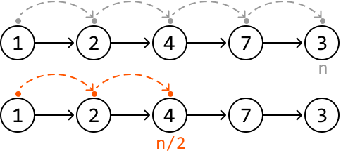
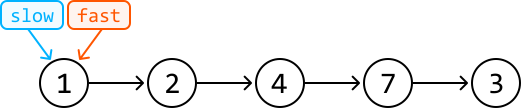
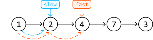

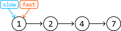
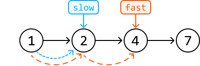


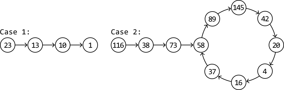
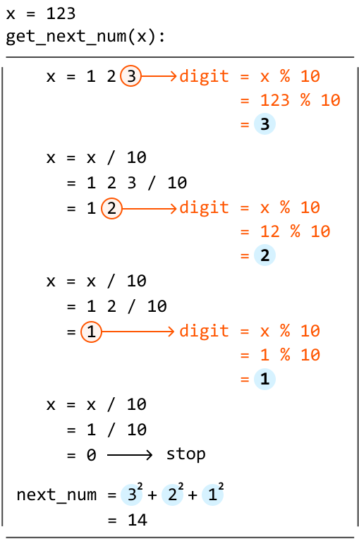
![The image represents a sliding window concept often used in algorithms. It shows a sequence of elements represented by dots enclosed in square brackets `[ . . . . . . ]`. A light-blue rectangular area highlights a subset of these elements, labeled 'window'. Two rectangular boxes, labeled 'left' and 'right,' are positioned above the sequence. A downward-pointing arrow connects 'left' to the leftmost dot within the window, and a similar arrow connects 'right' to the rightmost dot within the window. A light-blue upward-pointing arrow labeled 'window' indicates that this window can move along the sequence. The arrangement visually demonstrates how the window's position is controlled by the 'left' and 'right' pointers, allowing it to slide across the data sequence, processing a fixed-size subset at a time.](images/img_d11e8fd51c6c.svg)


![Image represents a visual depiction of a 'slide' operation in a data structure, likely an array or list. The left side shows an initial state with a light-blue, rounded-rectangle representing the data structure containing several black dots representing elements. Above this structure are two gray rectangular boxes labeled 'left' and 'right,' indicating the source of data insertion. Solid arrows point downwards from 'left' and 'right' to the leftmost and rightmost elements of the data structure, respectively. A horizontal arrow labeled 'slide' points to the right, separating the before and after states. The right side shows the data structure after the 'slide' operation. The light-blue rounded-rectangle again contains black dots, but now the 'left' and 'right' boxes are orange. Dashed orange arrows indicate that the 'left' and 'right' elements have been moved to the leftmost and rightmost positions, respectively, causing a shift in the other elements. The brackets '[' and ']' on both sides visually enclose the data structure, emphasizing its array-like nature. The overall diagram illustrates how elements are shifted within the data structure when a 'slide' operation is performed, with new elements potentially added at the beginning and end.](images/img_563c0f33d484.svg)


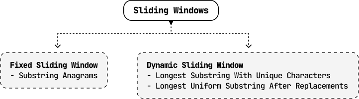





![Image represents a Python-like array assignment statement. The statement `expected_freqs = [...]` assigns a numerical array to the variable `expected_freqs`. The array is enclosed in square brackets `[]` and contains numerical values representing frequencies. Specifically, the first element is 2, associated with the character 'a'; the second is 1, associated with 'b'; the third is 0, associated with 'c'; and the remaining elements (indicated by an ellipsis '...') are all 0, extending up to and including the element associated with the character 'z'. The characters 'a' through 'z' are shown below the corresponding frequency values, indicating that the array likely represents the expected frequencies of each letter in the alphabet. There are no URLs or parameters present.](images/img_7cd76bbbc42c.svg)
![Image represents a data flow diagram illustrating a comparison process. On the left, two labeled boxes, 'left' and 'right,' point downwards with arrows to a light-blue rectangular box containing the character sequence 'c a a b a b'. This sequence appears to be a data window. To the right, the variable `window_freqs` is defined and assigned an array-like value `[2 0 1 ... 0]`, where the subscripts 'a', 'b', 'c', and 'z' indicate that the array represents the frequencies of characters 'a', 'b', 'c', and so on, up to 'z' within the window. The ellipsis (...) denotes that the array continues with frequencies for characters not explicitly shown. Below, a dashed-line box shows a comparison: `window_freqs != expected_freqs`, indicating that the calculated frequencies (`window_freqs`) are being checked against some pre-defined `expected_freqs`. An arrow labeled 'continue' emerges from this box, suggesting that the process continues if the comparison is true (i.e., the frequencies do not match the expected values).](images/img_225523d5e713.svg)
![Image represents a sliding window algorithm visualization. Two orange rectangular boxes labeled 'left' and 'right' point downwards with arrows to a light-blue rectangular box containing a sequence of characters 'c a a b a b'. Dashed lines extend from the arrows to indicate the window's boundaries. The 'left' pointer is positioned at the 'a' and the 'right' pointer at the 'b', defining the current window. Above, a list `window_freqs = [2 1 0 ... 0]` shows the frequency count of characters within the window (2 'a's, 1 'b', 0 'c', etc., up to 'z'). To the right, a light-grey box depicts a conditional check: `window_freqs == expected_freqs`, implying a comparison with a pre-defined frequency array (`expected_freqs`). If the condition is true, a counter `count` is incremented (`count += 1`). The diagram illustrates how the window moves across the character sequence, updating `window_freqs` and checking for matches against `expected_freqs` at each step.](images/img_2b012385f8aa.svg)
![Image represents a sliding window algorithm segment. Two orange rectangular boxes labeled 'left' and 'right' point downwards with arrows to a light-blue rectangular box containing the character sequence 'a b a'. Dashed arrows indicate the window's movement. The character 'c' precedes the window, and 'b' follows it. To the right, 'window_freqs = [2<sub>a</sub> 1<sub>b</sub> 0<sub>c</sub> ... 0<sub>z</sub>]' shows a frequency array; '2' indicates two occurrences of 'a' within the window, '1' shows one 'b', and '0' represents zero occurrences of 'c' and all other characters (represented by '...'). A light-grey dashed-line box displays the condition 'window_freqs == expected_freqs' which, if true, increments a counter: 'count += 1'. The diagram illustrates how the algorithm checks character frequencies within a sliding window against an expected frequency distribution ('expected_freqs'), updating a counter when a match is found.](images/img_9dae1e919b6f.svg)
![Image represents a sliding window algorithm visualization. Two orange rectangular boxes labeled 'left' and 'right' point downwards via orange arrows to a light-blue rectangular box containing the character sequence 'c a a b'. Dotted orange lines indicate the window's movement. Above, 'window_freqs = [1 2 0 ... 0]' shows an array representing the frequency of characters ('a', 'b', 'c', ..., 'z') within the current window, with 'a' having frequency 1, 'b' having frequency 2, and others having frequency 0. A light-grey dashed-line box displays the condition 'window_freqs != expected_freqs' and an arrow pointing right labeled 'continue,' indicating that if the window's character frequencies do not match the 'expected_freqs' (not shown), the algorithm continues processing. The overall diagram illustrates a step in a character frequency-based algorithm where a sliding window is used to compare observed frequencies against expected frequencies.](images/img_ece5db05933d.svg)
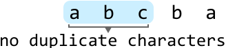
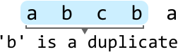
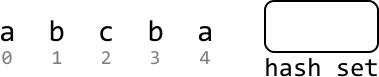







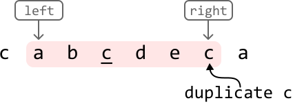
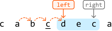
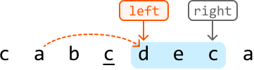
![Image represents a comparison of how a sliding window algorithm handles duplicate elements within and outside its current view. The diagram is split into two sections, each illustrating a scenario. The left section, titled 'Previous index inside the window:', shows a sequence 'cabcdeca' where a sliding window is highlighted, encompassing 'abcde'. Above this sequence, 'left' and 'right' boxes indicate the window's boundaries. Arrows point from these boxes to the 'a' at the left and 'c' at the right edge of the highlighted section. Below, a box displays the code `prev_indexes['c'] = 3 ≥ left`, indicating that the previous index of 'c' (3) is greater than or equal to the left boundary of the window (implied as 0), signifying that 'c' is already present within the window. Two arrows then point to the conclusions: 'inside window' and 'duplicate in the window'. The right section, titled 'Previous index outside the window:', shows a similar setup with the sequence 'cabcdeca', but the highlighted window is 'abc'. Again, 'left' and 'right' boxes point to the 'd' and 'a' respectively. The code `prev_indexes['a'] = 1 < left` shows that the previous index of 'a' (1) is less than the left boundary, meaning 'a' is outside the current window. Consequently, two arrows point to 'outside window' and 'not a duplicate in the window'. Both sections use color-coding: the highlighted window sections are shaded differently (pink/light blue) to distinguish the current window's contents, and the element being checked for duplication ('c' and 'a') is highlighted in a distinct color (peach/orange).](images/img_be854ee2d121.svg)



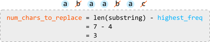
![Image represents a data flow diagram illustrating the process of finding the highest frequency of a character in a sequence. The input, shown as 'a b c' with a downward arrow indicating data flow, represents a sequence of characters. This input feeds into a table labeled 'freqs', which is a two-column table with headers 'char' and 'freq'. The table shows the character 'a' and its frequency '1'. This table acts as an intermediate data structure storing character frequencies. A separate box contains a code snippet: `highest_freq = max(highest_freq, freqs['a'])`, which calculates the highest frequency encountered so far. The variable `highest_freq` is updated using the `max` function, comparing its current value with the frequency of character 'a' (obtained from the `freqs` table using the key 'a'). The result of this calculation, '1', is displayed below the equation, indicating that the highest frequency found so far is 1. The overall diagram shows how the input sequence is processed to determine the highest character frequency.](images/img_48409481c723.svg)
![Image represents a data flow diagram illustrating a frequency counting algorithm. The input consists of a sequence of characters 'a', 'b', 'b', 'c', depicted by a downward-pointing arrow above the sequence. This input feeds into a table labeled 'freqs,' which is a two-column table with headers 'char' and 'freq.' The table stores the frequency of each character; 'a' has a frequency of 1, and 'b' has a frequency of 1. A separate, light-grey, dashed-bordered box contains a Python code snippet: `highest_freq = max(highest_freq, freqs['b'])`, which calculates the highest frequency encountered so far. The result of this calculation, `= 1`, is shown below the code snippet. The code implies an iterative process where `highest_freq` is updated by comparing it with the frequency of each character in the `freqs` table. The 'b' is used as an example in the code snippet, suggesting the algorithm iterates through each character in the input sequence.](images/img_b759196935b1.svg)
![Image represents a data flow diagram illustrating the process of finding the highest frequency of characters in a sequence. The input is a sequence of characters 'a b b c', depicted as a horizontal list. A downward arrow indicates this sequence is processed to generate a frequency table labeled 'freqs'. This table is a 2-column structure with the left column labeled 'char' representing characters and the right column labeled 'freq' representing their frequencies. The table shows 'a' with frequency 1 and 'b' with frequency 2. To the right, a separate box shows a Python-like code snippet calculating the highest frequency. The code `highest_freq = max(highest_freq, freqs['b'])` calculates the maximum frequency by comparing a current `highest_freq` (implicitly initialized to 0 or a lower value not shown) with the frequency of character 'b' (which is 2 from the table). The result, `= 2`, is displayed below, indicating that 2 is the highest frequency found in the input sequence.](images/img_95c20a169ab1.svg)
![Image represents a data flow diagram illustrating the process of finding the highest frequency of characters in a sequence. The input is a sequence of characters 'a b b c' shown with a downward arrow indicating data flow into a frequency table labeled 'freqs'. This table is a two-column structure with 'char' representing the character and 'freq' representing its frequency. The table shows 'a' with frequency 1, 'b' with frequency 2, and 'c' with frequency 1. To the right, a calculation is shown: `highest_freq = max(highest_freq, freqs['c']) = 2`. This equation indicates that the `highest_freq` variable is updated by taking the maximum value between its current value (implicitly assumed to be initialized to a value less than or equal to 2) and the frequency of character 'c' (which is 1 from the table), resulting in a final `highest_freq` value of 2. The diagram visually demonstrates how the frequency table is generated from the input sequence and how a maximum frequency is calculated using the table's data.](images/img_f3b8ba897705.svg)












![Image represents a visual depiction of a search space within a binary search algorithm. Two orange rectangular boxes labeled 'left' and 'right' are positioned above a horizontal line representing the 'search space'. This space contains a sorted array of integers: [1, 3, 4, 9, 10, 12, 14, 17, 20]. Arrows descend from 'left' and 'right' pointing to the beginning and end of the array, respectively. An orange line underneath the array is labeled 'search space,' indicating the range of values currently being considered during the search. The diagram illustrates the initial state of a binary search, where the algorithm is about to begin its search for a target value within the defined 'search space'.](images/img_d5cfb272f077.svg)





![Image represents two diagrams illustrating different loop termination conditions in a search algorithm, likely binary search. The left diagram shows a loop continuing 'while left < right', terminating 'once left == right'. Two orange rectangular boxes labeled 'left' and 'right' are positioned above a series of dots within square brackets [...], representing an array or list. Arrows descend from 'left' and 'right' pointing to separate dots within the array, suggesting the pointers are converging. The right diagram shows a loop continuing 'while left ≤ right', terminating 'once left > right'. Similarly, two orange boxes labeled 'right' and 'left' (note the order change) are above a series of dots within square brackets [...]. Arrows descend from 'right' and 'left', again pointing to separate dots within the array, but this time illustrating the pointers potentially crossing each other before termination. Both diagrams visually represent the iterative process of narrowing down a search space until a condition is met, highlighting the subtle difference in loop conditions and their impact on the final pointer positions.](images/img_dc77985dc1ce.svg)

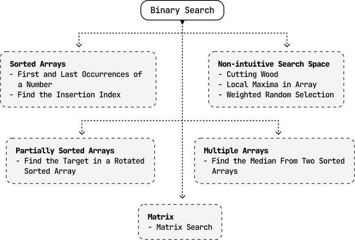
![Image represents two scenarios illustrating a search or insertion operation within a sorted integer array. The left side, titled 'case 1 - target exists in array:', shows an array `[1, 2, 4, 5, 7, 8, 9]` with indices displayed below each element (0-6). The target value, 4, is highlighted in a light green circle at index 2. The right side, titled 'case 2 - target not in array:', displays the array `[1, 2, 4, 5, 7, 8, 9]` with indices (0-6) similarly shown. Here, the target value is 6, which is not present. A light green circle highlights the index 4, indicating where the target value *would* be inserted to maintain the sorted order. A green upward-pointing arrow labeled 'insertion index' points to this highlighted index (4) in the second array. Both cases demonstrate how a target value's presence or absence affects the outcome of a search or insertion algorithm within a sorted array.](images/img_20459f205bcb.svg)
![Image represents a visual explanation of a conditional operation applied to an array. The top displays a conditional statement, `nums[i] >= target ?`, indicating a comparison where each element (`nums[i]`) of an array `nums` is checked against a `target` value. Below are two examples. Each example shows an array of numbers ([1, 2, 4, 5, 7, 8, 9]) and a specified `target` value (4 in the first example and 6 in the second). Underneath each array, a corresponding array of 'F' (False) and 'T' (True) values is shown. These boolean values represent the result of the comparison `nums[i] >= target` for each element. Grey downward-pointing arrows connect each element in the number array to its corresponding boolean value in the result array. In the first example (target = 4), elements less than 4 result in 'F', while elements greater than or equal to 4 result in 'T'. Similarly, in the second example (target = 6), elements less than 6 are 'F', and those greater than or equal to 6 are 'T'. The diagram illustrates how the conditional statement processes each array element to produce a boolean result array.](images/img_ab08055be20f.svg)
![The image represents two examples illustrating a lower bound in a data structure, likely an array. Each example shows a sequence enclosed in square brackets `[]`. The sequences consist of elements represented by 'F' (in red) and 'T' (in green). In both examples, a single 'T' element, highlighted within a light green circle, is positioned near the beginning of the sequence. An upward-pointing arrow originates from below this circled 'T' and points towards it, labeled 'lower bound'. The first example shows the sequence `[F F F T T T T T]`, while the second example shows `[F F F F F T T T]`. The arrangement demonstrates how the 'T' element acts as a lower bound, indicating a point in the sequence where the condition represented by 'T' begins to hold true. The difference between the two examples highlights that the exact position of the lower bound can vary depending on the data.](images/img_00f73d914d4b.svg)
![Image represents a visual depiction of a two-pointer approach to searching within a sorted array. Two rectangular boxes labeled 'left' and 'right' are positioned above a sorted integer array [1, 2, 4, 5, 7, 8, 9]. Arrows descend from 'left' and 'right' pointing to the beginning and end of the array respectively. The array elements are numbered below with their indices (0 to 7). To the right of the array, the text 'target = 4' indicates the value being searched for. The diagram illustrates the initial state of a binary search or similar algorithm where the 'left' pointer starts at index 0 and the 'right' pointer starts at index 6, preparing to search for the target value (4) within the array.](images/img_700b1c4202bc.svg)
![Image represents a visual depiction of a binary search algorithm step. Three rectangular boxes labeled 'left,' 'mid,' and 'right' are positioned above a numerical array [1, 2, 4, 5, 7, 8, 9], with each box pointing downwards via an arrow to its corresponding index in the array. The 'mid' box is highlighted in light blue, indicating its current focus. The number 4 in the array is highlighted in light green, representing the element at the 'mid' index. A dashed-line rectangle to the right displays a conditional statement: 'nums[mid] ≥ 4 → right = mid,' indicating that if the value at the middle index ('nums[mid]') is greater than or equal to 4, then the 'right' index is updated to the current 'mid' index. This illustrates a step in narrowing down the search space within the array. The numbers below the array represent the indices (0-7) of each element.](images/img_39a9f13d4d1f.svg)
![Image represents a visual depiction of a two-pointer approach in array traversal. A rectangular box labeled 'left' points down to a bracketed sequence `[1 2 4 5 7 8 9]`, indicating the starting point of a left pointer. The numbers are indexed below, starting from 0. A second rectangular box labeled 'right' points down to the number 5 within the sequence. A light-green circle highlights the number 4, visually separating the left and right pointers' initial positions. A dashed orange line curves from the number 5 (the right pointer's initial position) to the closing bracket `]`, suggesting the right pointer's traversal direction. The numbers 7, 8, and 9 are shown in lighter gray, indicating they are yet to be processed. The overall arrangement illustrates the initial state of a two-pointer algorithm operating on an array, where the left pointer starts at index 0 and the right pointer starts at index 3, with the right pointer moving towards the end of the array.](images/img_836fb2de31a7.svg)
![Image represents a visual depiction of a step within a binary search algorithm. Three rectangular boxes labeled 'left,' 'mid,' and 'right' are positioned above a numerical array [1, 2, 4, 5, 7, 8, 9], with index numbers displayed below each element. Arrows descend from 'left,' 'mid,' and 'right' pointing to the array elements 1, 2, and 5 respectively. The element at index 2 (value 4) is highlighted in light green. To the right, a dashed-line box contains a conditional statement: 'nums[mid] < 4 → left = mid + 1,' indicating that if the value at the middle index (nums[mid], which is 4 in this case) is less than 4, then the 'left' index should be updated to 'mid + 1'. This illustrates how the algorithm adjusts the search space based on the comparison of the middle element with the target value (implicitly 4 in this example).](images/img_f23ee289d435.svg)
![Image represents a visual depiction of a data structure manipulation, possibly illustrating an algorithm or a coding pattern. A horizontal line represents a sequence of numbered elements, bracketed by '[' and ']'. The numbers 1 through 9 are shown along this line, with numbers 0 through 7 displayed below as indices. A light green circle labeled '4' highlights an element within the sequence. Two rectangular boxes, one orange labeled 'left' and one gray labeled 'right', are positioned above the sequence. A solid orange arrow descends from 'left' pointing to the element '4', indicating a potential insertion or modification at that position. A solid gray arrow descends from 'right' pointing to the element '5', suggesting a similar action. A dashed orange curved line connects the 'left' box to the element '4', implying a possible search or selection process leading to the element '4' from the left side. The overall diagram likely illustrates how elements are accessed or manipulated within a sequence based on directional cues ('left' and 'right'), potentially demonstrating concepts like array indexing or list traversal.](images/img_3b30b912bda2.svg)
![Image represents a visual depiction of a step within a binary search algorithm. At the top, three rectangular boxes labeled 'left,' 'mid,' and 'right' are shown horizontally. Light blue arrows descend from 'mid' to highlight its index within a numerical array displayed below. This array, enclosed in square brackets `[ ]`, contains the numbers 1, 2, 4, 5, 7, 8, 9, with their indices (0-7) shown faintly beneath. The number 4, at index 2, is highlighted with a light green circle. The array's element at the index indicated by 'mid' (which is 4) is being compared to the value 4. To the right, a light gray, dashed-bordered rectangle displays the conditional logic: `nums[mid] ≥ 4 → right = mid`, indicating that if the value at the middle index (`nums[mid]`) is greater than or equal to 4, then the 'right' index is updated to be equal to the 'mid' index. This illustrates a step in narrowing down the search space within the binary search.](images/img_7a74307ef3d0.svg)
![Image represents a visual depiction of a data structure, possibly an array or list, with elements numbered 1 through 9, enclosed within square brackets '[' and ']'. A light-green circle labeled '4' highlights the element at index 2. Two rectangular boxes, one labeled 'left' in gray and the other 'right' in orange, indicate directional pointers. A solid gray arrow points from 'left' to the circled '4', while a solid orange arrow points from 'right' to the circled '4'. A dashed orange curved arrow originates near the circled '4' and points back towards it, suggesting an iterative or cyclical process. The numbers below the main line represent the indices of the array elements, ranging from 0 to 7, corresponding to the elements above. The overall diagram illustrates a concept related to accessing or manipulating an element within a data structure, potentially within the context of algorithms like binary search or other pointer-based operations.](images/img_6136e2a442d8.svg)
![The image represents a visual depiction of a search for a target value within a numerical array. The top row displays an array of integers enclosed in square brackets: [1, 2, 4, 5, 7, 8, 9]. To the right, separated by a comma, is the text 'target = 6,' indicating that the goal is to find the number 6 within the array. The bottom row shows the indices of the array elements, ranging from 0 to 7, corresponding to each element's position. A light-green circle highlights the index '4' which is below the number '7' in the array, suggesting that the algorithm is currently examining or has examined this element during its search for the target value 6. The absence of the target value (6) in the array is implicitly shown by the highlighting of an index that does not correspond to the target value.](images/img_828fb36c9575.svg)
![Image represents a visual depiction of a binary search algorithm step. Three rectangular boxes labeled 'left,' 'mid,' and 'right' are positioned above a numerical array [1, 2, 4, 5, 7, 8, 9], with each box pointing downwards via an arrow to its corresponding element's index in the array. The 'mid' box is highlighted in light blue, indicating its current focus. Below the array, indices 0 through 7 are displayed. The element at index 4 (value 7) is highlighted in light green. A dashed-line rectangular box contains the conditional statement 'nums[mid] < 6 → left = mid + 1,' illustrating that if the value at the middle index ('nums[mid]') is less than 6, the 'left' index is updated to 'mid + 1,' effectively narrowing the search space to the right half of the array for the next iteration. The arrows visually represent the data flow and the conditional logic of the algorithm.](images/img_245b0e4fdb7e.svg)
![Image represents a visual depiction of a data structure, possibly an array or list, illustrating a coding pattern. A numerical sequence [1, 2, 4, 5, 7, 8, 9] is displayed, with numbers positioned along a horizontal axis labeled with indices 0 through 7 below. An orange dashed line curves from a point between 1 and 2, reaching a point above the number 7. An orange rectangle labeled 'left' is connected by a downward-pointing arrow to the number 7. A gray rectangle labeled 'right' is connected by a downward-pointing arrow to the number 9. A light green circle containing the number 4 is positioned below the number 7, possibly indicating an index or a specific element's value. The dashed line suggests a connection or operation involving the 'left' pointer and the element at index 4, potentially illustrating a search or traversal algorithm within the data structure.](images/img_55556da2e12c.svg)
![Image represents a visual depiction of a step within a binary search algorithm. The top shows three labeled boxes: 'left,' 'mid' (highlighted in cyan), and 'right.' Arrows descend from 'left' and 'mid' pointing to the numbers 7 and 8 respectively, within a numerical array [1, 2, 4, 5, 7, 8, 9]. The array's indices are shown below, with index 4 highlighted in light green, corresponding to the value 7. An arrow descends from 'right' to the number 9 in the array. A separate, light-grey, dashed-bordered box displays the conditional logic: 'nums[mid] ≥ 6 → right = mid,' indicating that if the element at the middle index (`mid`) is greater than or equal to 6, then the 'right' index is updated to the value of `mid`. This illustrates how the algorithm adjusts the search space based on the comparison of the middle element with a target value (implicitly 6 in this case).](images/img_20105f753387.svg)
![Image represents a visual depiction of a coding pattern, likely illustrating array indexing or pointer manipulation. A numbered array, represented by `[1 2 4 5 7 8 9]`, is shown with indices displayed below (0-7). Two rectangular boxes labeled 'left' (gray) and 'right' (orange) point downwards to array elements 7 and 8 respectively. A downward-pointing arrow from 'left' indicates selection of element 7, while a similar arrow from 'right' points to element 8. A dashed orange curved line connects 'right' to the array's closing bracket `]`, suggesting a potential iteration or traversal to the end of the array. A small light green circle containing the number 4 is positioned below the element 7, possibly indicating an additional variable or index value related to the 'left' pointer. The overall arrangement suggests a scenario where two pointers, 'left' and 'right,' operate on the array, potentially for searching, sorting, or other array-processing algorithms.](images/img_b2505e277460.svg)
![Image represents a visual depiction of a step within a binary search algorithm. A numerical array `[1, 2, 4, 5, 7, 8, 9]` is shown, with indices displayed below. Three labeled boxes, 'left,' 'mid' (highlighted in cyan), and 'right,' are positioned above the array, indicating pointers or indices. Arrows from 'left,' 'mid,' and 'right' point downwards to the elements 7, 7, and 8 respectively in the array. The element at index 4 (value 7) is highlighted in light green, suggesting it's the current `mid` point. A separate, dashed-bordered box displays a conditional statement: `nums[mid] ≥ 6 → right = mid`, indicating that if the value at the `mid` index (7 in this case) is greater than or equal to 6, then the `right` pointer is updated to the `mid` index's value. This illustrates a decision-making step within the algorithm's iterative process of narrowing down the search space.](images/img_0560664ac32c.svg)
![Image represents a visual depiction of a binary search algorithm operating on a sorted array. A numbered array [1, 2, 4, 5, 7, 8, 9] is shown, with numbers 0 through 7 displayed below as indices. A light green circle labeled '4' indicates the midpoint of the array after an initial search. Two rectangular boxes, one labeled 'left' in gray and the other 'right' in orange, point downwards with arrows to the number '7' within the array. The 'left' arrow indicates a search starting from the left side of the array, while the 'right' arrow indicates a search from the right. A dashed orange arrow from 'right' to '7' shows the right pointer converging on '7'. This illustrates how the algorithm iteratively narrows down the search space by comparing the target value (implicitly understood to be 7) with the middle element, adjusting the search boundaries ('left' and 'right' pointers) until the target is found.](images/img_940a71c7d917.svg)
![Image represents a visual depiction of a binary search algorithm's step. At the top, a code snippet shows the conditional statement `if nums[mid] ≥ target: right = mid;`, indicating that if the element at the middle index (`mid`) of the array `nums` is greater than or equal to the target value, the `right` boundary of the search space is updated to `mid`. Below, two arrays, `[1, 2, 4, 5, 7, 8, 9]` and `[1, 2, 4, 5, 7, 8, 9]`, represent the initial and updated search spaces respectively. Index numbers are shown below each element. Boxes labeled 'left,' 'mid,' and 'right' indicate the boundaries of the search space. Arrows show the flow of information: 'left' points to the first element (index 0), 'mid' points to the element at index 3 (value 5), and 'right' initially points to the last element (index 7). In the updated array, a dashed orange line connects the previous `right` pointer (index 7) to the new `right` pointer (index 3), visually representing the narrowing of the search space due to the condition being met. The element at `mid` (value 5) is highlighted, and the number 4 is highlighted in both arrays to emphasize its position relative to the `mid` and `left` pointers.](images/img_3adcc438dca9.svg)
![Image represents a visual depiction of a binary search algorithm's iteration. The top shows a code snippet: `if nums[mid] < target: left = mid + 1`, indicating a conditional statement within the algorithm where if the value at the middle index (`mid`) of the array `nums` is less than the target value, the `left` boundary is updated to `mid + 1`. Below, two arrays `[1, 2, 4, 5, 7, 8, 9]` are shown, representing the search space. The first array shows the initial state with index numbers (0-7) beneath each element. Arrows labeled 'left,' 'mid,' and 'right' point to the respective boundaries of the search space (1, 5, and 9 initially). The second array illustrates the next iteration. The `mid` pointer has moved, and the `left` pointer has shifted to the right (indicated by an orange dashed arrow) because the condition `nums[mid] < target` was true. The `right` pointer remains unchanged. The index numbers are again shown below the array. The number 8 is highlighted in light green in both arrays, suggesting it might be the target value or relevant to the search.](images/img_13a17822ae1b.svg)
![Image represents a sequence of integers from 1 to 11, displayed in two rows. The top row shows the integers [1, 2, 3, 4, 4, 4, 5, 6, 7, 8, 9, 10, 11], with the three consecutive '4's highlighted in a light peach/orange rectangle. The bottom row displays the corresponding indices, ranging from 0 to 12. Two orange downward-pointing arrows connect the bottom row to labels below. The arrow originating from index 3 points to the label 'lower bound,' and the arrow originating from index 5 points to the label 'upper bound,' indicating that the highlighted sequence of three '4's starts at the lower bound (index 3) and ends at the upper bound (index 5).](images/img_3e48974fe854.svg)
![Image represents a visual depiction of a step within a binary search algorithm or a similar search/sorting process operating on a numerical array. The array `nums` is displayed horizontally, with elements [1, 2, 3, 4, 4, 4, 5, 6, 7, 8, 9, 10, 11]. Index values are shown below each element (0-12). Three labeled pointers, 'left', 'mid', and 'right', indicate array boundaries or positions. 'left' points to the beginning of the array (index 0), 'right' points to the end (index 12), and 'mid' points to element 4 at index 3 (highlighted in light green). A dashed box below the array displays a conditional statement: `nums[mid] > 4`. An arrow indicates that if this condition is true, then the 'right' pointer is updated to `right = mid - 1`, effectively narrowing the search space to the left half of the array. The visual arrangement clearly shows the pointers' positions and how the condition affects the 'right' pointer's movement, illustrating a key step in a divide-and-conquer approach to searching or sorting.](images/img_68f7c7c94dbb.svg)

![Image represents a visual depiction of a binary search algorithm's step. Three labeled boxes, 'left,' 'mid,' and 'right,' point downwards to respective indices within a numbered array [1, 2, 3, 4, 4, 4, 5, 6, 7, 8, 9, 10, 11]. The array's indices are shown below the numbers, ranging from 0 to 12. 'left' points to index 0 (value 1), 'mid' points to index 2 (value 3), highlighted in light green, and 'right' points to index 5 (value 4). A dashed box at the bottom displays the condition `nums[mid] < 4`, which evaluates to true because 3 < 4. An arrow indicates this condition leads to the assignment `left = mid + 1`, updating the 'left' index to 3 (the next index after 'mid'). The visual emphasizes the iterative process of narrowing down the search space within the array based on the comparison of the middle element with the target value (implicitly 4).](images/img_694cdf95fdcb.svg)

![Image represents a visual depiction of a binary search algorithm step. At the top, three rectangular boxes labeled 'left,' 'mid' (highlighted in light blue), and 'right' indicate index pointers. Arrows descend from each box, pointing to a numbered sequence [1, 2, 3, 4, 4, 4, 5, 6, 7, 8, 9, 10, 11] displayed below. The numbers are positioned above their corresponding indices (0-12) shown in a lighter gray. The 'mid' pointer points to the value '4' at index 4. A light green circle highlights the '4' at index 3, visually representing the 'left' pointer's position. The 'right' pointer also points to a '4' at index 5. At the bottom, a dashed-line box displays the code snippet 'nums[mid] == 4 → right = mid,' illustrating the algorithm's logic: if the value at the middle index ('nums[mid]') equals the target value (4), then the 'right' pointer is updated to the 'mid' index. This signifies that the search space has been narrowed down.](images/img_5fe4edc54966.svg)

![Image represents a visual depiction of a binary search algorithm step. A numbered array [1, 2, 3, 4, 4, 4, 5, 6, 7, 8, 9, 10, 11] is shown with indices displayed below. Three labeled boxes, 'left,' 'mid,' and 'right,' represent pointers to array elements. A light-green circle highlights the element at index 3, which is the value 4, indicating the current 'mid' point. Arrows point from 'left' and 'right' to the 'mid' element, showing how these pointers converge. Below the array, a code snippet 'nums[mid] == 4 → right = mid' illustrates the algorithm's logic: if the value at the midpoint ('nums[mid]') equals the target value (4), the 'right' pointer is updated to the current 'mid' index, effectively narrowing the search space to the left half of the array for the next iteration.](images/img_0fb9f1245ac2.svg)

![Image represents a visual depiction of a binary search algorithm step. At the top, three rectangular boxes labeled 'left,' 'mid' (highlighted in light blue), and 'right' are shown. Arrows descend from each box, pointing to elements within a numbered array represented horizontally below. The array, indexed from 0 to 12, contains the numbers [1, 2, 3, 4, 4, 4, 5, 6, 7, 8, 9, 10, 11]. The 'left' arrow points to the number 4 at index 3, the 'mid' arrow points to the number 4 at index 4, and the 'right' arrow points to the number 4 at index 5 (highlighted in light green). At the bottom, a gray dashed box displays the code snippet 'nums[mid] == 4 -> left = mid,' indicating that because the value at the middle index ('mid') is equal to 4, the 'left' index is updated to equal the 'mid' index. This illustrates a step in the binary search where the target value (4) has been found at the middle index, resulting in an update of the search space.](images/img_2e50010e25e8.svg)

![Image represents a visual depiction of a binary search algorithm step. A numbered array [1, 2, 3, 4, 4, 5, 6, 7, 8, 9, 10, 11] is shown, with indices displayed below. Above the array, three rectangular boxes labeled 'left,' 'mid,' and 'right' represent pointers or indices within the array. A light-green circle highlights the element at index 4 (value 4). Arrows point from 'left' and 'right' to this highlighted element, indicating the current midpoint of the search. Below the array, a code snippet 'nums[mid] == 4 → left = mid' shows that the value at the midpoint (nums[mid]) is 4, and consequently, the 'left' pointer is updated to equal the 'mid' pointer. This suggests the algorithm is searching for a value (likely 4), and this step shows the narrowing of the search space by updating the 'left' pointer.](images/img_60042666b465.svg)

![Image represents a visual depiction of a binary search algorithm step. At the top, three rectangular boxes labeled 'left,' 'mid,' and 'right' represent index pointers within a sorted numerical array shown below. The array, depicted as a number line from 0 to 12, contains the numbers 1 through 11. A light green circle highlights the element at index 4, which holds the value 4. Light blue arrows point from 'mid' to this highlighted element, indicating that the midpoint of the search is currently at index 4. Below the array, a dashed box displays the code snippet 'nums[mid] == 4 -> left = mid,' illustrating that because the value at the midpoint (nums[mid]) equals the target value (4), the 'left' pointer is updated to equal the 'mid' pointer. This signifies that the search has successfully found the target value at the midpoint.](images/img_c6e6c69015bd.svg)
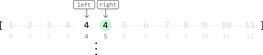


![Image represents a visual depiction of a step within a binary search algorithm. At the top, three rectangular boxes labeled 'left,' 'mid' (highlighted in light blue), and 'right' are shown. Arrows descend from each box, pointing to elements within a numbered array visualized horizontally below. The array contains the numbers 1 through 11, with indices displayed below. The 'left' arrow points to the number 4 at index 3, the 'mid' arrow points to the number 4 at index 4, and the 'right' arrow points to the number 4 at index 5 (highlighted in light green). At the bottom, a dashed-line box displays the code snippet 'nums[mid] == 4 → left = mid,' indicating that because the value at the middle index ('mid') of the array is equal to 4, the 'left' index is updated to be equal to the 'mid' index. This illustrates a key step in the binary search where the search space is narrowed based on the comparison of the middle element with the target value.](images/img_cfce1a2e35f2.svg)
![Image represents a visual depiction of a step within a binary search algorithm. A numbered array, indexed from 0 to 12, is shown with values implicitly represented by their index positions. The array segment from index 0 to 12 is displayed. Three labeled boxes, 'left' (orange), 'mid' (cyan), and 'right' (gray), represent index pointers. Arrows indicate that 'left' and 'right' initially point to indices 3 and 5 respectively, while 'mid' points to index 4. A light green circle highlights the element at index 4, which has a value of 4. A dashed orange arrow shows a tentative movement of the 'left' pointer. A solid cyan arrow shows the movement of the 'mid' pointer. A separate box displays the condition `nums[mid] == 4 -> left = mid`, indicating that because the element at the midpoint (index 4) equals 4, the 'left' pointer is updated to the value of the 'mid' pointer (index 4). This illustrates a step where the target value is found at the midpoint, resulting in the update of the 'left' pointer.](images/img_8f1295c0e265.svg)

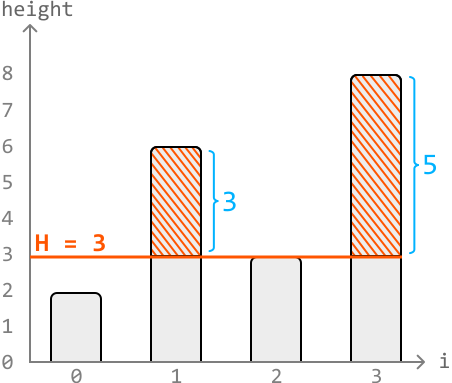
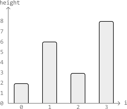
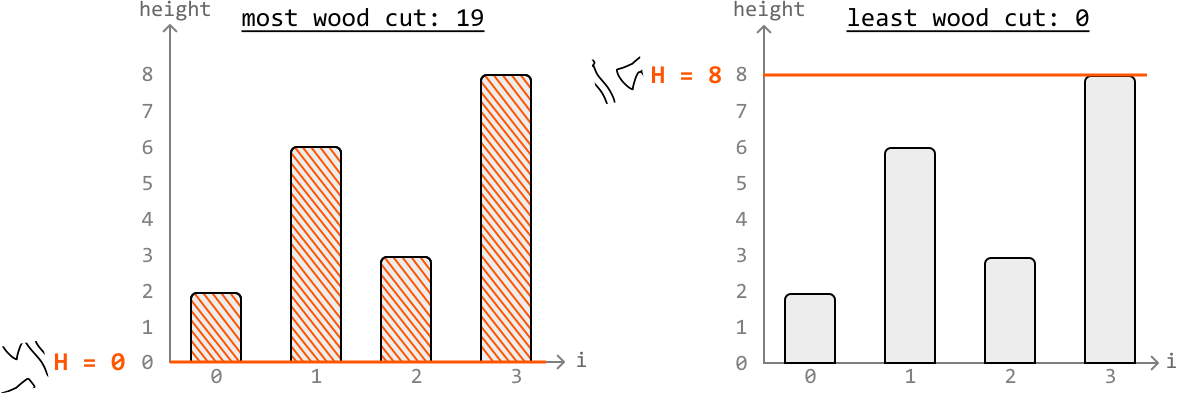
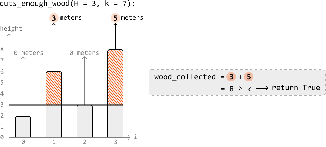



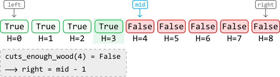

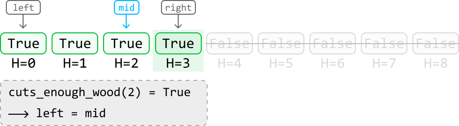

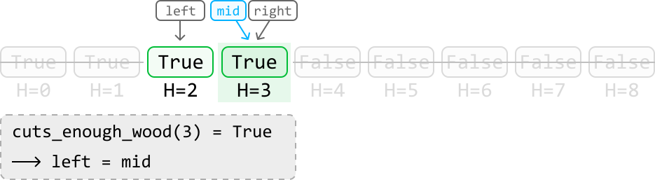

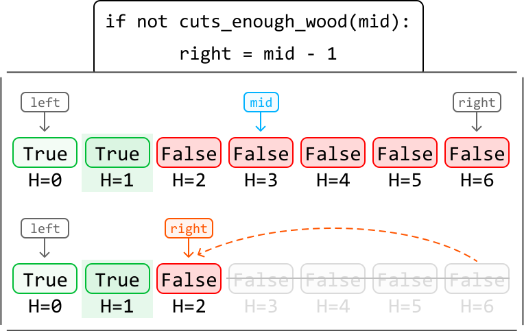
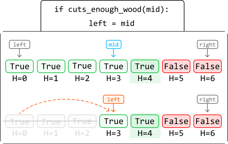
![Image represents a depiction of a search problem. The top row shows a list of integers, represented as an array `[8, 9, 1, 2, 3, 4, 5, 6, 7]`, enclosed in square brackets. This array is implicitly indexed, with the indices 0 through 8 shown in a smaller font below the corresponding array elements. The text 'target = 1' indicates that the goal is to find the element with the value 1 within the array. The arrangement visually suggests a linear search scenario, where the algorithm would sequentially check each element of the array until it finds the element matching the target value. There are no explicit connections or information flow depicted beyond the visual representation of the array and the target value.](images/img_5202a1f0d3a0.svg)
![Image represents a visual depiction of array partitioning, likely within the context of a divide-and-conquer algorithm. Three rectangular boxes labeled 'left' (orange), 'mid' (light blue), and 'right' (orange) are positioned above a numerical array [8, 9, 1, 2, 3, 4, 5, 6, 7]. Arrows descend from each box, pointing to the array elements. The 'left' box's arrow points to the first two elements (8 and 9), the 'mid' box's arrow points to the element 3 (the middle element in this example), and the 'right' box's arrow points to the last two elements (6 and 7). The numbers beneath the array (0-8) represent the indices of the array elements. The diagram illustrates how an array is conceptually divided into sections, possibly for recursive processing, with the 'mid' pointer potentially indicating a pivot point or a division boundary.](images/img_0e26cde300a4.svg)
![Image represents a visual depiction of a sorting algorithm, likely merge sort, illustrating the merging of two sorted subarrays. The top section shows an unsorted array [8, 9, 1, 2, 3, 4, 5, 6, 7] divided into three parts: 'left' [8, 9, 1, 2], 'mid' [3], and 'right' [4, 5, 6, 7]. Arrows labeled 'left', 'mid', and 'right' point downwards to their respective subarrays, indicating the input to the merging process. The bottom section displays a bar chart representing the same numbers. The 'left' subarray's bars are taller and unsorted, while the 'right' subarray's bars are shorter, light blue, and sorted in ascending order, as indicated by the label 'ascending' below the chart. The bars visually represent the magnitude of each number. The merging process is implied by the juxtaposition of the sorted 'right' subarray with the unsorted 'left' subarray, suggesting the next step would be to combine them into a single sorted array.](images/img_19f41316d70d.svg)
![Image represents a visual depiction of a two-pointer approach in a coding pattern, likely for array traversal or manipulation. A gray rectangular box labeled 'left' points down to a numerical array [8, 9, 1, 2, 3, 4, 5, 6, 7]. Below the array, gray numbers 0 through 8 indicate the indices. An orange rectangular box labeled 'right' points down to the element '2' in the array, signifying its initial position. A dashed orange line curves from the element '2' to the element '7', illustrating a connection or interaction between these two points. The numbers 3, 4, 5, 6, and 7 are shown in gray, indicating they are part of the array but not directly involved in the initial pointer positions. The overall diagram suggests a process where two pointers, one starting at the left and one at a position within the array, interact or move through the array, possibly to find a specific element or perform a comparison.](images/img_88aae002c194.svg)
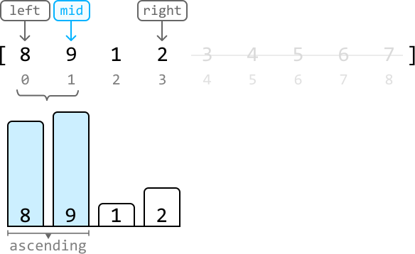
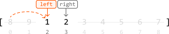
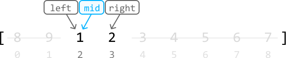
![Image represents a visual explanation of a binary search algorithm's behavior, specifically Case 1 where the subarray [left:mid) is sorted. The top section shows an initial array [3, 4, 5, 6, 7, 1, 2] represented as bars with their values labeled. Gray boxes labeled 'left' and 'right' indicate the initial search boundaries. A light-blue box labeled 'mid' highlights the middle element (6). A downward-pointing arrow from 'left' points to 3, and another from 'right' points to 2. A cyan arrow points from 'mid' to the element 6. The bottom-left shows pseudocode: `if nums[left] <= target < nums[mid] → right = mid - 1` else `→ left = mid + 1`. This logic dictates how the search boundaries ('left' and 'right') are adjusted based on the target value's relationship to the middle element. The bottom-right shows two subsequent steps of the algorithm. The first shows the array after the first iteration, with the 'right' pointer moved to the element 5. The second shows the array after the second iteration, with the 'left' pointer moved to the element 7. Gray curved arrows connect the pseudocode to these steps, illustrating how the algorithm updates the search space based on the condition. The dashed orange lines show the movement of the 'right' and 'left' pointers across the array during the iterations.](images/img_1d571af395ce.svg)
![Image represents a visual explanation of a coding pattern, specifically a case within a binary search algorithm. The top section shows an array of numbers [6, 7, 1, 2, 3, 4, 5] partitioned into three sections labeled 'left,' 'mid,' and 'right.' The 'mid' section (containing 2) is highlighted in light blue. Arrows indicate the boundaries of these sections. Below this, two further examples illustrate the algorithm's iterative steps. The first shows the 'left' pointer moving to the right, encompassing the 'mid' section, after a comparison. The second example shows the 'right' pointer moving to the left, after a different comparison. A gray box at the bottom contains pseudocode: `if nums[mid] < target < nums[right] → left = mid + 1` and `else → right = mid - 1`. This code describes the conditional logic determining the pointer movement based on the target value's relationship to the values at the 'mid' and 'right' indices. Curved arrows in orange and gray connect the array representations to show the pointer movements ('left' in orange, 'right' in gray) during the algorithm's iterations. The overall diagram demonstrates how the algorithm iteratively narrows the search space by adjusting the 'left' and 'right' pointers until the target is found or the search space is exhausted.](images/img_484e1375c490.svg)
![Image represents two Python list assignments. The first line assigns a list named `nums1` containing the integer elements 0, 2, 5, 6, and 8. The second line assigns a list named `nums2` containing the integer elements 1, 3, and 7. Both lists are presented using standard Python list notation, with square brackets `[]` enclosing the elements, and commas separating them. There is no explicit connection or data flow shown between the two lists; they are simply defined independently of each other.](images/img_6f1a429dd233.svg)
![Image represents a one-dimensional array labeled 'merged array:'. The array is enclosed in square brackets `[]` and contains the following integer elements, listed sequentially: 0, 1, 2, 3, 5, 6, 7, 8. There are no other visible components, connections, or information flows depicted in the image beyond the array itself and its descriptive label. The elements are presented without any apparent structure or organization beyond their numerical order within the array.](images/img_18877f214105.svg)
![Image represents a visual depiction of splitting an array into two halves. A numerical array, represented by elements [0, 1, 2, 3, 5, 6, 7, 8] enclosed in square brackets, is shown. A dashed-line box visually separates the array into a 'left half' (elements 0, 1, 2, 3) and a 'right half' (elements 5, 6, 7, 8). The element '4' is seemingly absent. The text 'left half' in cyan is positioned below the left half of the array, while 'right half' in orange is below the right half. Upward-pointing arrows connect the end of the left half (element 3) with the text 'end of left half' in cyan above it, and the start of the right half (element 5) with the text 'start of right half' in orange above it. This illustrates the division point and the labeling of the two resulting sub-arrays.](images/img_b08bfd409bc4.svg)
![Image represents a visual depiction of a partitioning algorithm, likely quicksort, showing the process of dividing an array into smaller sub-arrays. Three stages are shown, each displaying an array represented as two horizontal rows of numbers enclosed in square brackets `[]`. The top row contains elements `[0, 2, 5, 6, 8]` in all three stages, while the bottom row contains `[1, 3, 7]` which remains constant. The arrays are partitioned using two colored lines: light blue for the 'left partition' and light orange for the 'right partition'. Triangles (pointing upwards) indicate pivot points within each partition. Numbers above the lines indicate the lengths of the partitions. A curved arrow labeled 'slice' shows the movement of the partition boundaries, illustrating how the algorithm iteratively divides the array. The legend clarifies that the arrow indicates data movement from the right partition to the left partition. The initial array is implicitly divided into two partitions based on the pivot. Subsequent stages show the refinement of these partitions, with the final stage suggesting a nearly sorted array.](images/img_c7aa8aabdc17.svg)
![Image represents a visual depiction of array splitting or partitioning. The top section shows two 2D arrays, one light blue containing the elements [0, 2] in the first row and [1, 3] in the second, and the other peach-colored containing [5, 6, 8] in the first row and [7] in the second. A vertical line separates these arrays. Light blue horizontal lines with small triangles at their ends indicate the lengths of the rows in the light blue array (2 elements in the top row and 2 in the bottom). Similarly, orange lines with triangles show the lengths of the rows in the peach array (3 elements in the top row and 1 in the bottom). The numbers '2' and '3' above the arrays indicate the lengths of the respective rows. The bottom section displays the same elements arranged as two 1D arrays: a light blue array [0, 1, 2, 3] and a peach array [5, 6, 7, 8], separated by a vertical line, representing the concatenated elements from the original 2D arrays. The diagram illustrates how a larger array might be conceptually divided into smaller sub-arrays, potentially for parallel processing or other algorithmic purposes.](images/img_bb9690f6a004.svg)
![Image represents a diagram illustrating a coding pattern, likely related to array or list comparisons. The diagram shows two rectangular regions, one light blue and one peach, representing potentially two different arrays or lists. Each region contains several black dots representing elements, and two circled elements labeled L1, L2 (light blue) and R1, R2 (peach). L1 and L2 are positioned at the right edge of their respective regions, while R1 and R2 are positioned at the left edge of their respective regions. A horizontal line connects the right edge of the light blue region to the left edge of the peach region. The text below the diagram specifies a condition to be checked: `(L1 ≤ R1, L1 ≤ R2)` and `(L2 ≤ R1, L2 ≤ R2)`. This indicates a comparison where the values of L1 and L2 (from the light blue region) are checked to see if they are less than or equal to the values of R1 and R2 (from the peach region). The brackets `[` and `]` around the elements suggest that the regions represent ordered sequences, possibly arrays or lists.](images/img_0c3066948e9d.svg)
![Image represents three examples illustrating a coding pattern, possibly related to array partitioning or range checks. Each example shows a numerical array enclosed in square brackets, partitioned into sub-arrays. The first array in each example is split into two sub-arrays, with the partitioning point indicated by a vertical line. Numbers within the array are represented by circles; light blue circles represent the lower bounds of sub-arrays, and peach circles represent upper bounds. Below each example is a small box containing two inequality checks. The first example shows the array `[1, 3, 5, 6, 8]` partitioned at `5`, with checks `5 ≤ 3` (false, marked with 'x') and `1 ≤ 6` (true, marked with '✓'). The second example shows `[1, 3, 2, 5, 7]` partitioned at `2`, with checks `2 ≤ 7` (true, '✓') and `3 ≤ 5` (true, '✓'). The third example shows `[-∞, 1, 3, 6, 8]` partitioned at `6`, with checks `6 ≤ 1` (false, 'x') and `-∞ ≤ 8` (true, '✓'). The pattern appears to involve checking inequalities based on the partitioning point and elements within the sub-arrays.](images/img_a91cff43b068.svg)
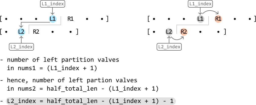
![Image represents a visual depiction of a coding pattern, possibly related to array manipulation or indexing. Three rectangular boxes labeled 'left,' 'L1_index,' and 'right' point downwards to an array [0, 2, 5, 6, 8]. The number 5 is highlighted in light blue and labeled 'L1,' indicating a left index or pointer. Below this array, a sub-array [0, 3, 7] is shown, with 3 highlighted in light orange and labeled 'R2,' suggesting a right index or pointer. A dashed rectangular box contains the equation 'L1 > R2 → right = L1_index - 1,' illustrating a conditional statement: if the value at the left index (L1) is greater than the value at the right index (R2), then the 'right' variable is updated to be one less than the value of 'L1_index.' The diagram visually demonstrates the relationship between array indices, pointers, and a conditional update based on their values.](images/img_b3e340222656.svg)
![Image represents a diagram illustrating a coding pattern, possibly related to array manipulation or searching. The diagram shows two arrays, labeled L1 and L2, represented as `[0 2 5 6 8]` and `[0 3 7 +∞]` respectively. The number 2 in L1 and 7 in L2 are highlighted in peach and light blue respectively, and labeled R1 and R2. Three rectangular boxes above L1 contain the labels 'left', 'L1_index', and 'right'. Arrows point from 'left' and 'L1_index' to the beginning of L1, indicating these variables might be used to index or access elements within L1. A dashed-line box displays the equation 'L2 > R1 → left = L1_index + 1', suggesting a conditional operation: if an element in L2 (specifically R2) is greater than an element in L1 (specifically R1), then the 'left' variable is updated to the value of 'L1_index' plus 1. This implies an iterative process where the 'left' index is adjusted based on comparisons between elements of L1 and L2. The '+∞' in L2 suggests a sentinel value or a boundary condition.](images/img_1e9470c864e3.svg)
![Image represents a diagram illustrating a coding pattern related to array slicing. At the top, a rectangular box labeled 'left L1_index right' points downwards with arrows to two sets of data. The first set is an array represented as `[0 2 5 6 8]`, where '2' is highlighted in light blue and labeled 'L1', and '5' is highlighted in light orange and labeled 'R1'. Below this, a second array `[0 3 7]` is shown, with '3' highlighted in light blue and labeled 'L2', and '7' highlighted in light orange and labeled 'R2'. A dashed rectangular box on the right states the condition 'L1 ≤ R2 and L2 ≤ R1' which, if true (indicated by a right-pointing arrow), results in a 'correct slice'. The diagram visually demonstrates how the indices 'L1', 'R1', 'L2', and 'R2' from two arrays are compared to determine if a slice is valid based on the condition.](images/img_4ae4a78c5d10.svg)
![Image represents a visual explanation of a merge sort algorithm step. Two arrays, `[0 2 5 6 8]` and `[0 3 7]`, are shown, with their elements visually separated by a vertical line. Light blue circles highlight the numbers 2 and 3 in the respective arrays, indicating these are the largest element in the left array and the smallest element in the right array, respectively. A curved arrow points from the 3 to indicate that it's the smallest element on the right, and another curved arrow points to the 3 from the left to indicate that it's the largest element on the left. An orange circle highlights the number 5 in the right array, indicating it's the smallest element in that array. Below, a merged array `[0 1 2 3 5 6 7 8]` is displayed, showing the result of merging the two input arrays in sorted order. The numbers 1 and 2 are implicitly understood to be part of the merged array, as they are the next smallest elements after 0. The diagram illustrates the process of selecting the smallest element from the right array and the largest element from the left array during the merging phase of the merge sort.](images/img_79e8aa17a850.svg)
![Image represents a demonstration of merging two sorted arrays. The top line shows an array named `nums1` containing the integer elements [0, 2, 5, 6, 8]. The second line displays another array, `nums2`, with elements [1, 3, 7, 9]. Below these, labeled 'merged array:', is the result of merging `nums1` and `nums2` into a single sorted array: [0, 1, 2, 3, 5, 6, 7, 8, 9]. The elements from `nums1` are shown in black, while elements from `nums2` are displayed in light blue and orange, illustrating their origin within the merged array. There are no URLs or parameters present; the image solely depicts the data structures and the outcome of the merging operation.](images/img_13f83ff7a6ec.svg)
![Image represents a partially merged array visualized during a merge sort algorithm. The text 'merged array:' labels a numerical array represented within square brackets `[]`. The array contains elements colored in two different colors: `0`, `1`, `2`, and `3` are displayed in cyan, while `5`, `6`, `7`, `8`, and `9` are in orange. A vertical bar `|` and brackets `[]` highlight the number `5` within the orange section. An orange curved arrow points from the text 'start of right half' to the highlighted `5`, indicating that this element represents the beginning of the right half of an array that is being merged with a left half (represented by the cyan numbers). The overall image illustrates a step in the merge sort process where the algorithm is combining sorted sub-arrays.](images/img_490f583c2636.svg)
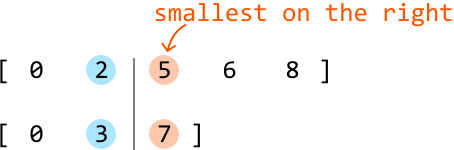
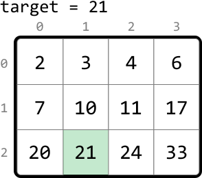
![Image represents a data transformation process visualized using a matrix and arrows. A 3x4 matrix is shown, with rows labeled 0, 1, and 2, and columns labeled 0, 1, 2, and 3. Each cell in the matrix contains a numerical value (2, 3, 4, 6, 7, 10, 11, 17, 20, 21, 24, 33). Light orange arrows indicate data flow. Two arrows originate from the top-left corner of the matrix, one from row 0 and one from row 1, pointing downwards to a horizontal array below the matrix. This array displays the values from the first two rows of the matrix, concatenated horizontally ([2, 3, 4, 6, 7, 10, 11, 17]). A third arrow originates from the right side of the matrix, pointing downwards to another horizontal array, which displays the values from the last row of the matrix, concatenated horizontally ([20, 21, 24, 33]). The final output is a single horizontal array containing all the values from the matrix, arranged sequentially.](images/img_aa466b4a22b1.svg)
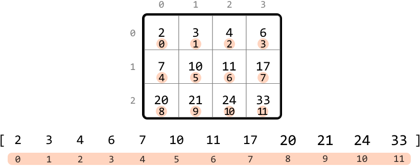
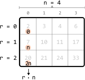
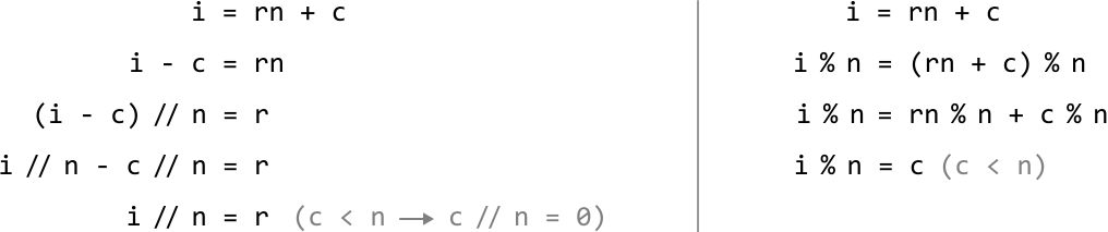
![Image represents a visual explanation of a search algorithm within a 4x4 matrix. The top shows 'target = 21,' indicating the value being searched for. A 4x4 matrix is displayed below, with each cell containing a number and its row and column index shown as subscripts. The matrix is labeled with 'left', 'mid', and 'right' indicating index pointers. The 'mid' pointer highlights the value 10 at row 1, column 1. To the right, calculations are shown: 'r = mid // n' (integer division of 'mid' by 4, resulting in 1) and 'c = mid % n' (modulo operation of 'mid' by 4, resulting in 1). This determines the row (r=1) and column (c=1) of the element to check. The condition 'matrix[r][c] < target' (10 < 21) is shown, indicating that the element at row 1, column 1 is less than the target. Finally, the consequence 'left = mid + 1' is shown, suggesting the algorithm updates the 'left' pointer based on the comparison result. The highlighted cell (21) shows the target value found in the matrix.](images/img_bf5017836b5c.svg)
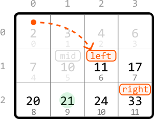
![Image represents a visual explanation of a search algorithm within a 4x4 matrix. The top shows 'target = 21,' indicating the value being searched for. A 4x4 matrix is displayed below, with rows labeled 0, 1, 2 and columns labeled 0, 1, 2, 3. Each cell contains a number, and the cell containing 20 is labeled 'mid' (in cyan), the cell containing 11 is labeled 'left' (in orange), and the cell containing 33 is labeled 'right' (in orange). To the right, a separate box details the calculation process: 'r = mid // n' (integer division of mid by n, where mid is 8 and n is 4, resulting in r=2) and 'c = mid % n' (modulo operation of mid by n, resulting in c=0). The line 'matrix[r][c] < target' indicates a comparison between the value at matrix position [2][0] (which is 20) and the target value (21). The result of this comparison (20 < 21) leads to the assignment 'left = mid + 1,' implying an adjustment of the search range based on the comparison. The overall diagram illustrates a step in a binary search or similar algorithm applied to a 2D array.](images/img_fa38b10bca85.svg)
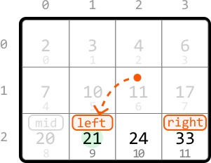
![Image represents a visual explanation of a search algorithm within a 4x4 matrix. The top shows 'target = 21,' indicating the value being searched for. A 4x4 matrix is displayed below, with each cell containing a number and its row and column indices subtly indicated. The matrix's rows are indexed 0, 1, and 2, and columns are indexed 0, 1, 2, and 3. The number 21 is highlighted within the matrix, labeled 'left,' indicating its position in the search. To its right is the number 24, labeled 'mid,' and to its further right is 33, labeled 'right.' These labels suggest a binary search-like approach. A separate box to the right details the calculation process: 'r = mid // n' and 'c = mid % n' calculate the row (r) and column (c) indices of the 'mid' element (24 in this case), where 'mid' is 10 (its index in a flattened array), 'n' is 4 (the number of columns). The calculations show r = 2 and c = 2. Finally, 'matrix[r][c] > target → right = mid - 1' indicates that if the value at matrix[2][2] (which is 24) is greater than the target (21), the right boundary of the search is updated to 'mid - 1', effectively narrowing the search space.](images/img_bc754fa76530.svg)
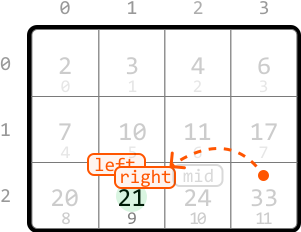
![Image represents a visual explanation of a search algorithm within a matrix. A 3x4 matrix is shown, with each cell containing a number and its index (row, column) subtly displayed below. The top row displays column indices (0, 1, 2, 3), and the leftmost column displays row indices (0, 1, 2). The number 21 is highlighted within the matrix at index (2,1), indicating a 'mid' value. To the right, a separate box details the calculation: `r = mid // n` (integer division of `mid` (9) by `n` (4), resulting in `r = 2`) and `c = mid % n` (modulo operation of `mid` (9) by `n` (4), resulting in `c = 1`). This calculation determines the row (`r`) and column (`c`) indices of the element being checked. Finally, the condition `matrix[r][c] == target` is shown, indicating that if the element at the calculated index (`matrix[2][1]`) equals the `target` value (21), the function returns `True`. The overall diagram illustrates how a search algorithm might locate a target value within a matrix using integer division and modulo operations to determine the index.](images/img_b422124e4de7.svg)
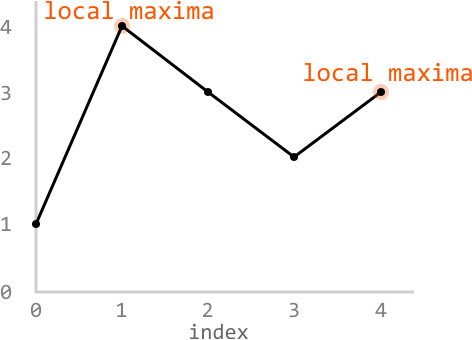
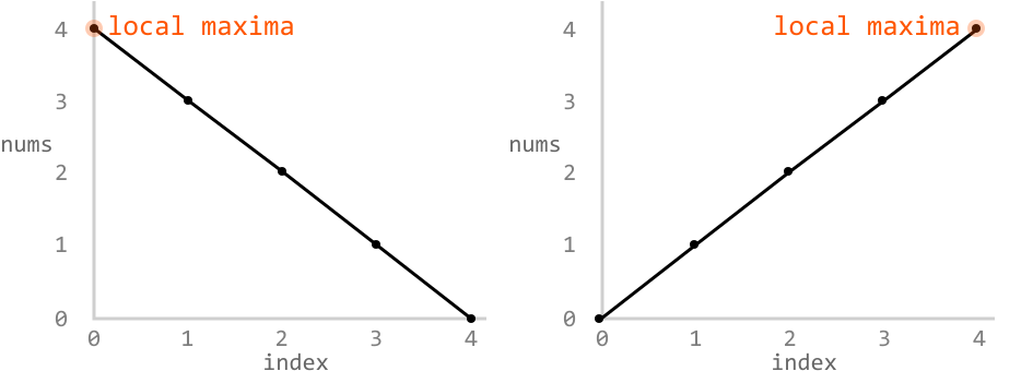
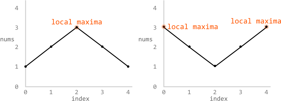
![Image represents a diagram illustrating a condition within a coding pattern, likely related to finding local maxima in an array. Two orange circles represent array indices 'i' and 'i+1', with downward-pointing orange arrows indicating access to the corresponding array elements `nums[i]` and `nums[i+1]`. A thick black line connects the circle representing 'i' to a black dot representing an intermediate state. A dashed line extends from this dot, suggesting a continuation. An orange arrow points from 'i+1' to this black dot. The text `nums[i] < nums[i+1]` indicates a comparison between the values at these indices. A rightward arrow follows this comparison, leading to the text 'local maxima somewhere to the right of i,' implying that if the condition `nums[i] < nums[i+1]` is true, a local maximum is expected to exist at some index greater than 'i'. The overall diagram visually represents the logic flow of checking for an increasing trend in the array to potentially identify a local maximum.](images/img_972fd2489e71.svg)
![Image represents a diagram illustrating a condition for identifying local maxima within a numerical sequence represented by the array `nums`. The diagram features two nodes, one colored orange and the other black, connected by a solid black arrow pointing from the orange node to the black node. Above the orange node, a downward-pointing orange arrow labeled 'i' indicates an index `i` in the `nums` array. Similarly, a downward-pointing orange arrow labeled 'i+1' points to the black node, representing the next index `i+1`. A dashed line extends from a point slightly to the left and above the orange node, suggesting a continuation of the sequence before index `i`. The core logic is expressed as `nums[i] > nums[i+1]`, indicating that if the value at index `i` is greater than the value at index `i+1`, then either a local maximum exists somewhere to the left of index `i`, or the value at `nums[i]` itself is a local maximum. The text to the right of the inequality explains these two possible outcomes.](images/img_f0be01010287.svg)
![Image represents a line graph illustrating a numerical array. The horizontal axis is labeled 'index' and ranges from 0 to 6. The vertical axis is labeled 'nums' and ranges from 0 to 4. A black line connects data points representing the values of an array [0, 1, 4, 2, 1, 2, 3], where each number corresponds to its index. The array is displayed above the graph. Two orange vertical lines highlight the leftmost (index 0, value 0) and rightmost (index 6, value 3) elements of the array. Above these lines, orange rectangular boxes labeled 'left' and 'right' respectively, indicate the boundaries. The area under the line graph is filled with a light peach color.](images/img_595d1eac3175.svg)
![Image represents two line graphs illustrating a coding pattern, likely a binary search algorithm. Both graphs display the same data points: `[0, 1, 4, 2, 1, 2, 3]` plotted against an index from 0 to 6. The y-axis represents the 'nums' values. In both graphs, vertical orange lines mark 'left' and 'right' boundaries, and a light-blue arrow indicates 'mid'. The left graph shows the initial state with 'left' at index 0, 'mid' at index 3, and 'right' at index 6. A shaded peach area highlights the section between 'left' and 'right'. The right graph depicts an iteration where a descending slope is detected (nums[mid] > nums[mid + 1]), resulting in 'right' being updated to the 'mid' index (index 3). A dashed orange line connects the old and new 'right' positions. A grey box in the left graph explains the condition for updating 'right' in the algorithm: `descending slope: nums[mid] > nums[mid + 1] → right = mid`. A small arrow points from this box to the right graph, indicating the application of this rule.](images/img_7edfaa941c44.svg)
![Image represents a visual explanation of a coding pattern, likely within a sorting or searching algorithm. The image is divided into two nearly identical parts, each showing a line graph with a series of points connected by lines. The x-axis represents an index (0-6), and the y-axis represents numerical values ('nums'). In both parts, orange vertical lines highlight sections of the graph. Above each graph, rectangular boxes labeled 'left,' 'mid,' and 'right' indicate index values (e.g., [0 1 4 2 1 2 3] in the first part) that are associated with the graph's points. Arrows point from these boxes down to their corresponding points on the graph. A dashed gray line connects the 'left' and 'right' indices in the second part, suggesting a range. A light peach-colored rectangle highlights a section of the graph between the 'left' and 'right' markers. A separate box explains the condition 'ascending slope: nums[mid] < nums[mid + 1] → left = mid + 1,' indicating that if the value at the midpoint is less than the value at the next point, the 'left' index is updated to the midpoint plus one. This suggests an iterative process of narrowing down a search range based on the slope of the line graph. The two parts likely illustrate different stages of this iterative process.](images/img_a29edcf3af44.svg)
![Image represents a visual explanation of a coding pattern, likely within a binary search algorithm. The image is divided into two nearly identical halves, each showing a line graph plotting a numerical array `nums` against its index. The x-axis represents the index (0 to 6), and the y-axis represents the values within the `nums` array. Both graphs depict the same data, a series of points connected by lines forming a V-shape. At the top of each half, labeled boxes indicate pointers `left`, `mid`, and `right`, initially pointing to indices 0, 2, and 3 respectively in the left half and 0, 1, and 3 in the right half. These pointers define a search window within the array. A shaded orange vertical bar highlights the `mid` index in the left graph. A gray box in the left half explains a condition: 'descending slope: nums[mid] > nums[mid + 1] → right = mid,' indicating that if the value at `mid` is greater than the value at `mid + 1`, the `right` pointer is updated to `mid`, effectively narrowing the search space. The right half likely shows the result of applying this condition, with the `right` pointer moved to index 1. The overall diagram illustrates how the algorithm iteratively refines the search range based on the slope of the data.](images/img_74a83945d6c5.svg)
![Image represents a visual explanation of a step within a binary search algorithm, specifically illustrating a condition where the middle element is greater than the element to its right. The image is divided into two parts separated by a large right-pointing arrow. The left part shows an array `[0, 4, 3, 1, 0]` represented graphically as a line graph with the x-axis representing the index (0 to 4) and the y-axis representing the array's values (0 to 4). Vertical orange lines mark the `left` (index 0), `mid` (index 2), and `right` (index 4) pointers, with corresponding labels above the lines. A shaded peach area highlights the section of the array between `left` and `right`. A black line connects the data points, showing the array's values. The right part shows the updated state after the condition `if nums[mid] > nums[mid + 1]: right = mid;` is executed. The `right` pointer has moved from index 4 to index 2, indicated by a dashed orange line connecting the old and new positions. The graph is updated to reflect this change, with the new `right` pointer at index 2. Above both parts, a code snippet displays the condition `if nums[mid] > nums[mid + 1]: right = mid;`, which is the decision-making logic behind the pointer movement. The overall image demonstrates how the algorithm adjusts its search space based on the comparison of the middle element with its neighbor to the right.](images/img_9668bf7da6f5.svg)
![Image represents a visual explanation of a coding pattern, likely within a sorting algorithm. The top shows a code snippet: `if nums[mid] < nums[mid + 1]: left = mid + 1;`, indicating a conditional statement comparing two elements of an array `nums` at indices `mid` and `mid + 1`. Below, a line graph displays an array `nums` = [0, 4, 3, 1, 0] with indices 0-4 on the x-axis and values on the y-axis. Orange vertical lines mark `left` (index 0), `mid` (index 2), and `right` (index 4), initially. A shaded peach region highlights the section between `left` and `right`. A black line connects the data points. A grey dot marks the `mid` point's value. A thick black arrow separates this from a second graph showing the array after the conditional statement's execution. In the second graph, `left` has shifted to index 3, indicated by a new orange line, while `right` remains at index 4. The peach shaded region now reflects the updated `left` and `right` boundaries. The dashed orange line connects the old and new `left` positions, visually demonstrating the shift. The second graph's line plot remains the same, but the `left` pointer's position has changed, illustrating the algorithm's step in adjusting the search space based on the comparison.](images/img_2eb3a081084b.svg)
![Image represents a Python code snippet assigning a list of weights. The snippet shows the variable `weights` being assigned a list containing two numerical values: 1 and 4. The assignment is represented using the equals sign (`=`). The list is denoted by square brackets (`[` and `]`). The numbers 0 and 1 are faintly visible below the numbers 1 and 4 respectively, possibly indicating indices or positions within the list. There is no other information, such as URLs or parameters, present in the image. The overall structure is a simple variable assignment statement common in programming languages.](images/img_9b939dc59d06.svg)
![Image represents a simple illustration of weight normalization in a context likely related to machine learning or weighted averaging. The top line shows a Python-like variable assignment, `weights = [1 4]`, defining a weight vector with two elements: 1 and 4. Below, these weights are individually depicted with small downward arrows pointing to their normalized counterparts. The normalization appears to be a simple division by the sum of the weights (1+4=5). Therefore, the weight 1 is transformed into 1/5 (displayed in cyan), and the weight 4 is transformed into 4/5 (displayed in orange). The small numbers '0' and '1' above the arrows likely represent indices indicating the position of each weight within the original vector. The overall diagram visually demonstrates the process of converting a set of weights into their normalized probability distribution.](images/img_607824cc0639.svg)


![Image represents a visual depiction of weighted indexing. At the top, a list named 'weights' is defined as an array containing the integers [3, 1, 2, 4]. Below this, a horizontal bar is segmented into four color-coded sections, each labeled 'index 0,' 'index 1,' 'index 2,' and 'index 3,' respectively. The bar is further divided into numbered units from 1 to 10. Colored arrows connect the weights to the bar; a cyan arrow from the weight '3' points to the end of the 'index 0' section (at position 3), a green arrow from the weight '1' points to the end of the 'index 1' section (at position 4), an orange arrow from the weight '2' points to the end of the 'index 2' section (at position 6), and a magenta arrow from the weight '4' points to the end of the 'index 3' section (at position 8). Each arrow's length visually represents the corresponding weight value, indicating how many units each index occupies within the bar. The numbers above the arrows (0, 1, 2, 3) correspond to the index of the weight in the `weights` array.](images/img_7f791e39e2c8.svg)
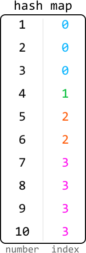

![Image represents a visual depiction of an array, specifically a one-dimensional array or list. The array is enclosed in square brackets `[` and `]`. The array contains four elements: 3, 4, 6, and 10. These elements are displayed horizontally, separated by spaces. Below each element, in a lighter gray font, is an index indicating its position within the array. The indices start from 0 and increment sequentially: 0 for the element 3, 1 for the element 4, 2 for the element 6, and 3 for the element 10. The arrangement clearly shows the mapping between each element's value and its corresponding index within the array's structure.](images/img_96469211dc66.svg)


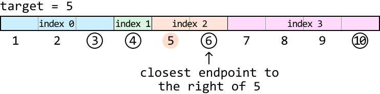
![Image represents a depiction of prefix sums, showing an array `prefix_sums` initialized with values [3, 4, 6, 10]. The array is presented horizontally. Each element's value is displayed numerically. Below each element, a colored vertical line indicates its status: 'F' (in red) represents 'False', and 'T' (in green) represents 'True'. The first two elements (3 and 4) are marked with 'F', while the last two elements (6 and 10) are marked with 'T'. This suggests a visual representation of a boolean condition applied to the prefix sums, where the last two elements satisfy the condition and the first two do not. The arrangement visually links the numerical value of each element with its corresponding boolean status.](images/img_8c3750aa3746.svg)
![Image represents a visual depiction of a two-pointer approach to finding a subarray with a target sum. Two orange rectangular boxes labeled 'left' and 'right' point downwards towards an array represented by `prefix_sums = [3, 4, 6, 10]`. Beneath each element of the `prefix_sums` array, its index (0, 1, 2, 3) is shown in gray. The number 6 in the `prefix_sums` array is highlighted in light green. A separate line indicates `target = 5`. The arrows from 'left' and 'right' visually suggest the movement of pointers across the `prefix_sums` array during the algorithm's execution, aiming to find a subarray whose sum equals the `target` value. The highlighted '6' likely represents a point where the algorithm might find a solution (or a relevant intermediate state), given that the difference between consecutive prefix sums could be used to determine the sum of subarrays.](images/img_00fa3871b72c.svg)
![Image represents a visual depiction of a binary search algorithm's step within the context of prefix sums. The diagram shows four labeled boxes: 'left,' 'mid,' and 'right' representing index pointers, and a dashed box containing a conditional statement. 'left' and 'mid' point downwards to an array [3, 4, 6, 10] with indices 0, 1, 2, and 3 respectively displayed below each element. 'right' also points downwards to the same array. Below the array, 'target = 5' is specified. The dashed box displays the condition 'prefix_sums[mid] < target,' which evaluates whether the prefix sum at the 'mid' index is less than the target value (5). If true, as indicated by the arrow, the 'left' pointer is updated to 'mid + 1,' effectively narrowing the search space in a binary search fashion. The light blue box around 'mid' and the blue arrow visually emphasize the current 'mid' index and its role in the conditional statement.](images/img_6ec25c663f14.svg)
![Image represents a visual depiction of a binary search algorithm's step. A sorted array `[3, 4, 6, 10]` is shown with indices 0, 1, 2, and 3 labeled below each element. A light gray rectangle labeled 'mid' points to the element '4' at index 1. An orange rectangle labeled 'left' points to the element '6' at index 2. A dark gray rectangle labeled 'right' points to the element '10' at index 3. A dashed orange line connects the 'mid' label to the element '3' at index 0, indicating a comparison. A solid orange arrow points from 'left' to '6', showing the selection of the left subarray. A solid dark gray arrow points from 'right' to '10', showing the selection of the right subarray. The arrangement visually demonstrates the partitioning of the array during a binary search iteration, with the 'mid' element acting as the pivot for comparison and subsequent subarray selection.](images/img_0e1643066d92.svg)
![Image represents a visual depiction of a binary search algorithm step within a coding pattern context. The top shows three labeled boxes: 'left,' 'mid' (highlighted in cyan), and 'right.' Arrows point downwards from 'left' and 'right' to the array [3, 4, 6, 10], indicating index positions 0, 2, and 3 respectively. The 'mid' box points to the element '6' at index 2. Below the array, 'target = 5' is specified. A dashed box to the right shows a conditional statement: 'prefix_sums[mid] ≥ target,' which evaluates whether the prefix sum at the midpoint (6 in this case) is greater than or equal to the target (5). A right-pointing arrow from this condition leads to the assignment 'right = mid,' indicating that if the condition is true, the right boundary of the search space is updated to the midpoint. The overall diagram illustrates a single iteration of a binary search, where the algorithm checks if the prefix sum at the midpoint meets or exceeds the target value to refine the search range.](images/img_0693ad8ea34d.svg)
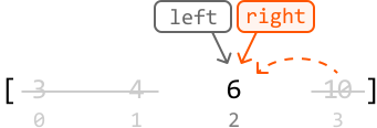
![Image represents a diagram illustrating a coding pattern, possibly related to binary search or a similar algorithm. At the top, two orange rectangular boxes labeled 'left' and 'right' are shown, with downward-pointing arrows indicating data flow. Below, a horizontally oriented array or list is depicted, showing the elements [3, 4, 6, 10] with their indices [0, 1, 2, 3] displayed underneath. The 'left' and 'right' labels appear to represent pointers or indices into this array. The arrows from 'left' and 'right' point to the element '6' in the array, suggesting that these pointers are converging on a specific element. To the right, a light gray, dashed-line rectangle contains the conditional statement 'left == right' followed by a right-pointing arrow and the action 'return left'. This indicates that if the left and right pointers are equal, the algorithm returns the value at the left pointer's index. The overall diagram visualizes a search or comparison process where two pointers move towards each other until they meet, at which point a result is returned.](images/img_4462fc41d123.svg)
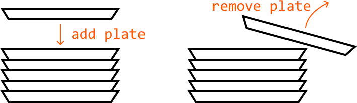
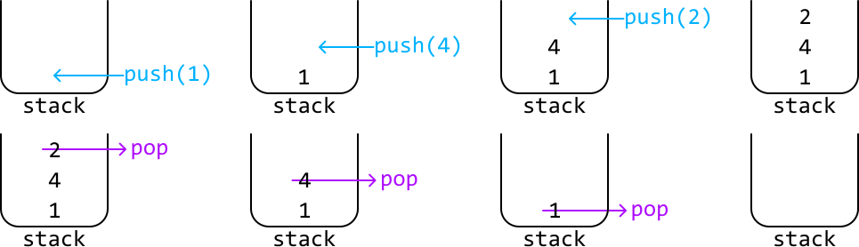
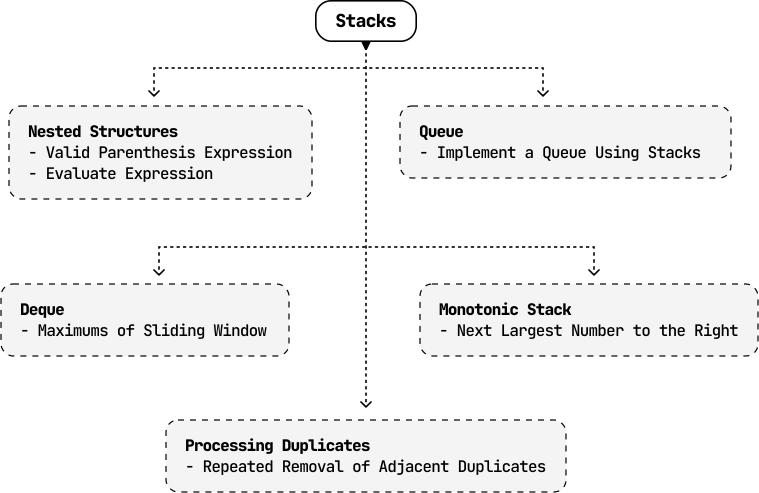
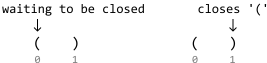
![Image represents a comparison of two scenarios illustrating parenthesis matching in a coding context. The left side depicts a correctly matched sequence, showing the text 'most recent parenthesis waiting to be closed' above a gray downward-pointing arrow. This arrow points to a sequence of parentheses: `[(])`, indexed 0 to 3 from left to right. The closing parenthesis at index 3 correctly matches the opening parenthesis at index 1, indicating proper nesting. In contrast, the right side shows an incorrectly matched sequence. The text 'does not close most recent parenthesis' (in red) is positioned above a red downward-pointing arrow, which points to a similar sequence `[(])`, also indexed 0 to 3. However, here the closing parenthesis at index 3 does *not* match the most recent opening parenthesis (at index 1), highlighting an error in parenthesis matching. Both sides use the same parenthesis characters and indexing to facilitate a direct comparison of correct versus incorrect parenthesis closure.](images/img_ce94423dc115.svg)
![Image represents a sequence of six distinct symbols, arranged horizontally from left to right with spaces between them. The symbols are: an opening parenthesis `(`, an opening square bracket `[`, a closing square bracket `]`, an opening curly brace `{`, a closing parenthesis `)`, and a closing curly brace `}`. There are no connections or information flow depicted between the symbols; they are simply presented as individual, independent elements. No labels, text, URLs, or parameters are present within the image. The image likely illustrates the different types of grouping symbols used in programming languages or mathematical notation.](images/img_4e0b08bd6e2d.svg)
![Image represents a visual explanation of a stack data structure used for parenthesis matching. On the left, a sequence of opening and closing parentheses, brackets, and braces – `( [ ] { } )` – is shown, with an orange square containing an 'i' and a downward arrow pointing to the sequence, suggesting input. On the right, a diagram depicts a stack labeled 'stack' with a 'top' indicator. A light-grey 'top:' label points to the top of the stack, which is currently empty. A light-blue arrow labeled 'push (' indicates that the opening parenthesis '(' is being pushed onto the stack, implying that the algorithm is processing the input sequence from left to right and using the stack to keep track of opening delimiters. The overall image illustrates the initial step of a parenthesis matching algorithm using a stack.](images/img_fca6200b86f2.svg)
![Image represents a visual explanation of a stack data structure used in coding, specifically demonstrating a push operation. On the left, a sequence of opening and closing parentheses, brackets, and braces: `( [ ] { ) }` is shown. An orange square containing an 'i' symbol, suggesting input, points downwards with an arrow towards the '[' bracket, indicating the element being processed. On the right, a diagram depicts a stack labeled 'stack' with a 'top' pointer. The stack currently contains an opening parenthesis '('. A light-blue arrow labeled 'push [' shows the '[' bracket being added to the top of the stack, illustrating the 'push' operation where a new element is added to the top of the stack. The arrangement visually explains how an input element is added to the stack, modifying its contents and updating the top pointer.](images/img_73ad5fbd1851.svg)
![Image represents a visual explanation of a stack data structure used for parenthesis matching. On the left, a sequence of opening and closing parentheses, brackets, and braces — `(`, `[`, `]`, `{`, `)` — is shown. An orange square labeled 'i' points downwards, indicating an input stream of these characters. To the right, a stack is depicted as a container labeled 'stack' with a 'top' pointer indicating the top element. Inside the stack, an opening bracket '[' is present. A purple arrow labeled 'pop' extends from the top of the stack to a light gray dashed box containing the text ''[' is closed by ']':', illustrating that the top element '[' is being popped from the stack, implying a matching closing bracket ']' is expected in the input stream to maintain balanced parentheses. The diagram demonstrates how a stack is used to verify the correct pairing of opening and closing delimiters in a given input string.](images/img_4c2893503dbb.svg)
![Image represents a visual explanation of a stack data structure and its 'push' operation. The left side shows a sequence of opening and closing brackets and braces: '(', '[', ']', '{', ')', '}'. A downward-pointing orange arrow with a small orange square containing an 'i' (likely indicating information or instruction) points to the '{' character. This suggests the '{' is the next element to be processed. The right side depicts a stack labeled 'stack' with its contents shown as '{' and '('; the label 'top:' indicates the top of the stack. A light-blue arrow labeled 'push { ' points from the right to the stack, illustrating the 'push' operation where the '{' character is being added to the top of the stack. The overall diagram demonstrates how a character ('{') is pushed onto a stack, which is a Last-In, First-Out (LIFO) data structure.](images/img_feeb5e542720.svg)
![Image represents a visual explanation of a stack-based approach to validating balanced parentheses in a code snippet. On the left, a sequence of opening and closing parentheses, brackets, and braces (`(`, `[`, `{`, `)`, `]`, `}`) is shown. An orange arrow with an 'i' icon points downwards towards the curly brace '{' and closing parenthesis ')'. To the right, a diagram depicts a stack data structure labeled 'stack,' with the characters '{' and '(' currently inside it, indicating that these opening brackets have been pushed onto the stack. The label 'top:' points to the top of the stack, which is '{'. A light gray dashed-line box contains pseudocode: `'{' is not closed by ')': return False`, illustrating a scenario where an opening curly brace '{' is encountered, but its corresponding closing brace '}' is not found before a closing parenthesis ')', resulting in a `False` return value, indicating unbalanced parentheses. The overall image demonstrates how a stack can be used to track opening brackets and check for proper closing counterparts during code validation.](images/img_3ae5aab44183.svg)
![Image represents a simple diagram titled 'parenthesis_map' illustrating a mapping between opening and closing parentheses, brackets, and braces. The diagram is rectangular and divided vertically into two equal sections labeled 'open' and 'closed' respectively. The 'open' section displays an opening curly brace '{', an opening square bracket '[', and an opening parenthesis '(', stacked vertically. The 'closed' section mirrors this, showing the corresponding closing curly brace '}', closing square bracket ']', and closing parenthesis ')', also stacked vertically in the same order. The arrangement visually demonstrates a one-to-one correspondence between each opening symbol on the left and its respective closing symbol on the right, implying a data structure or algorithm that relies on pairing these symbols for validation or processing.](images/img_0599becd83ae.svg)
![The image represents a bar chart illustrating a data transformation or accumulation process. The horizontal axis displays an unsorted sequence of numerical values (5, 2, 4, 6, 1), each represented by a black vertical bar whose height corresponds to its magnitude. Below the chart, a list `res = [6 4 6 -1 -1]` shows the resulting data after some operation. Dashed orange arrows connect the tops of the bars to corresponding values in the `res` list, indicating a mapping or transformation. For instance, the bar representing '5' maps to '6' in the `res` list, the bar representing '2' maps to '4', and so on. The vertical axis represents the magnitude of the values, ranging from 0 to 6. The chart visually demonstrates how the input values are processed to produce the output values in the `res` list, suggesting a potential algorithm involving accumulation or modification of the input sequence. The negative values in `res` suggest a possible subtraction or other negative transformation applied to some input values.](images/img_944d4e732575.svg)
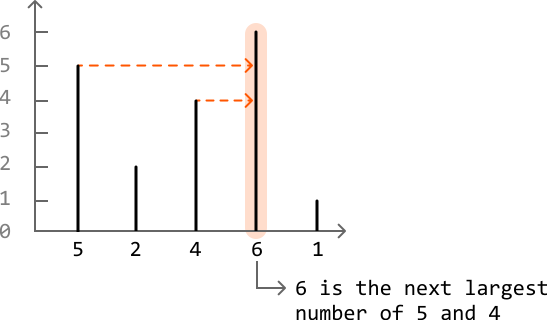
![Image represents a bar chart illustrating a frequency distribution. The horizontal axis displays a sequence of numbers: [1, 1, 2, 3, 2, 3, 2, 4], representing data points. The vertical axis represents frequency, ranging from 0 to 4. Above each number on the horizontal axis, a vertical bar extends upwards to a height corresponding to its frequency of occurrence within the sequence. For instance, the number '1' appears twice, thus its bar reaches the height of '1' on the vertical axis; the number '2' appears three times, resulting in its bar reaching the height of '2'; the number '3' appears twice, reaching the height of '2'; and the number '4' appears once, reaching the height of '4'. The chart visually summarizes the frequency of each unique value in the given data set.](images/img_fb53777c8749.svg)
![Image represents a Cartesian coordinate system illustrating a data structure or algorithm, possibly related to candidate selection or a similar process. The horizontal axis depicts an array or list, labeled `[ ... 4 ]` at its ends, suggesting a sequence of elements where '4' is the last visible element, and ellipses (...) indicate unseen preceding elements. The vertical axis represents a numerical value or index, ranging from 0 to 4. A vertical line segment extends from the horizontal axis at the point labeled '4' to the top of the diagram, indicating a selection or operation focused on the element '4'. To the right, the text `candidates = []` shows an empty array or list named 'candidates', suggesting this structure might store selected elements. The text `res = []` similarly shows an empty array named 'res', likely representing the results or output of the process. The downward-pointing arrow above the vertical line suggests data flow or an operation being performed on the element '4'. The overall diagram likely visualizes a step in an algorithm where the element '4' is being processed or selected, with the 'candidates' and 'res' arrays potentially storing intermediate or final results.](images/img_ff99a340c9e9.svg)
![Image represents a Cartesian coordinate system illustrating a step in a coding pattern, possibly related to backtracking or a similar algorithm. The horizontal axis represents an index or iterator, with values implicitly ranging from an unspecified starting point to 4, indicated by the label `[... 4]`. The vertical axis represents a value or counter, ranging from 0 to 4. A vertical line segment extends from the horizontal axis at the point x=4, reaching a value of approximately 4 on the y-axis. To the right of the coordinate system, the text `candidates = [4]` indicates a list or array named `candidates` containing the single element 4. Below this, `res = [-1]` shows a list or array named `res` containing the single element -1, highlighted in a peach-colored box. The downward-pointing arrow above the vertical line suggests a process is occurring at index 4, potentially modifying the `res` array. The overall diagram likely visualizes a state within an iterative algorithm where the `candidates` list is being processed, and the `res` list is being updated.](images/img_1b4016b684d8.svg)
![Image represents a Cartesian coordinate system illustrating a step in a coding algorithm, possibly related to backtracking or dynamic programming. The horizontal axis shows a range of values, with labeled points at 2 and 4, implying a discrete domain. The vertical axis represents a count or index, ranging from 0 to 4. Two vertical lines are drawn at x=2 and x=4, extending from the horizontal axis to y=2 and y=4 respectively. A dashed orange arrow points from the line at x=2 to the line at x=4, indicating a transition or step in the algorithm. Below the horizontal axis, `res = [ ... 4 -1]` is shown, suggesting a result array or list where '4' (highlighted in peach) is a current value and '-1' might represent a placeholder or a special value. To the right, `candidates = [4 2]` is displayed, indicating a list of candidate values used by the algorithm. The overall diagram visualizes a process where the algorithm moves from a state represented by the line at x=2 to a state represented by the line at x=4, updating the `res` array in the process, using values from the `candidates` list.](images/img_454eae90c29e.svg)
![Image represents a graphical illustration of a filtering process within a coding pattern, likely related to candidate selection or data pruning. A horizontal axis displays a sequence of numbers, including 2, 3, and 4, representing candidate values. Vertical lines of varying styles indicate the presence and status of these candidates. A solid black vertical line at '3' and '4' signifies that these candidates are initially present. A dashed red vertical line at '2' shows it as a candidate that will be removed. A downward-pointing grey arrow above the '3' suggests a filtering operation is being applied. To the right, the text 'remove all candidates ≤ 3:' in red describes the filtering criterion, while 'candidates = [4 2]' shows the initial candidates, and 'candidates = [4]' shows the candidates after filtering. Below, 'res = [4 -1]' likely represents the result of a subsequent operation on the remaining candidates. The vertical axis likely represents a frequency or some other metric, but its scale is not explicitly defined. The overall diagram visually demonstrates the removal of candidates based on a specified condition, resulting in a filtered set of candidates.](images/img_9782984b2a9d.svg)
![Image represents a graphical depiction of a step in an algorithm, possibly related to candidate selection or a similar process. The core of the image is a Cartesian coordinate system with a horizontal x-axis and a vertical y-axis ranging from 0 to 4. Along the x-axis, a partially visible array `[ ... 3 2 4]` is shown, indicating a sequence of numbers. Two vertical lines, one black and one light gray, represent elements within this array. The black line is positioned at x=3 and extends vertically to y=3, while the light gray line is at x=2 and extends to y=1. A dashed orange arrow points horizontally from the top of the black line (at y=3) to a second black line positioned at x=4, extending vertically to y=4. Below the x-axis, the text `candidates = [4 3]` is displayed, suggesting these are the current candidates being considered. Additionally, `res = [ 4 4 -1]` is shown, likely representing the results or output of the algorithm so far, with the number 4 highlighted in a peach color. The downward-pointing gray arrow above the first black line indicates the current processing step. The overall diagram illustrates a transition or movement of data, possibly a value of 3, from one position in the array to another, updating the `candidates` and `res` arrays accordingly.](images/img_19e8e2b64e2e.svg)
![Image represents a bar graph combined with a line graph illustrating a coding pattern. The x-axis displays a sequence of numbers: [1, 1, 2, 3, 2, 3, 2, 4], representing an input array. Above each x-axis value, a vertical bar is drawn; the height of the bar corresponds to the values in a second array, `res = [2, 2, 3, 4, 3, 4, 4, -1]`, shown below the x-axis. The bars are black for positive values in `res` and light gray for the last value (-1). An orange line connects points representing a cumulative sum or another derived value from the `res` array. This line starts at (1,1) and increases with each subsequent point, indicating a trend. Separately, a rectangular box displays the array `candidates = [4, 3, 2, 1]`, which is labeled as 'decreasing,' indicating the array's elements are in descending order. An orange arrow points from the `candidates` array to the right, visually connecting it to the graph, suggesting that the `candidates` array is the input or a related data structure used to generate the graph's data.](images/img_a4db7c470bac.svg)


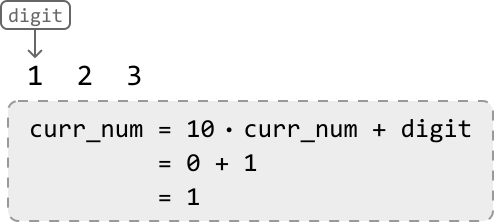
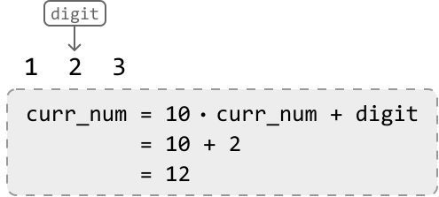
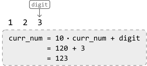







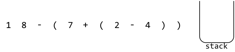





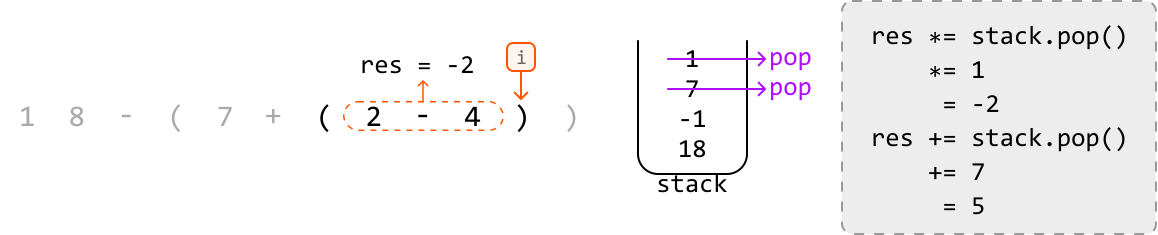
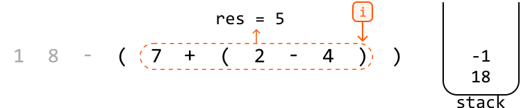
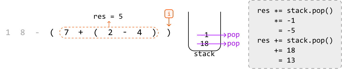
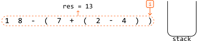



![Image represents a visual depiction of an algorithm, likely for string manipulation. The top section shows an input string 'a a c a b b a' preceded by a downward-pointing arrow originating from a square box labeled 'i,' suggesting an input indicator. This input string is then processed, resulting in a 'new string: a' displayed to the right. The bottom section mirrors the top, again showing the input string 'a a c a b b a' with the same input indicator 'i.' However, the resulting 'new string' is shown as 'a [a]' with a red line striking through the second 'a', indicating removal. A dashed-line box to the right of the bottom section labels this action as 'remove adjacent duplicate,' clarifying the algorithmic step performed. The overall diagram illustrates a process where adjacent duplicate characters are identified and removed from the input string.](images/img_0de1fa84b2cc.svg)
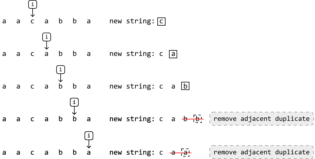
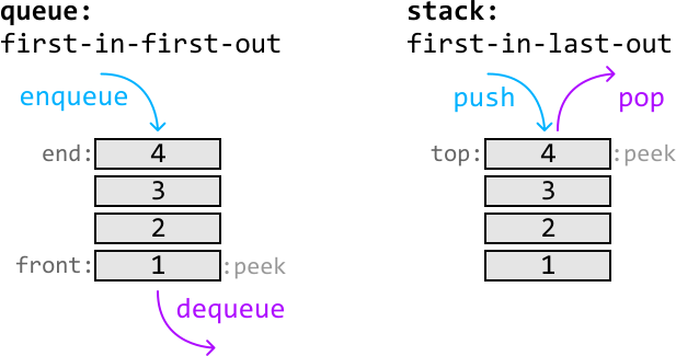

![Image represents a step-by-step visualization of a stack data structure's pop operation. Three diagrams show the stack's state at different points. Each diagram features a stack represented as a container with numbered elements (1, 2, 3) stacked vertically, with the top element indicated by 'top:'. A 'temp' array below each stack shows the elements popped so far. In the first diagram, a purple arrow labeled 'pop' shows the top element (3) being removed from the stack and added to the 'temp' array, which now contains [3]. The second diagram shows the next pop operation, with the top element (2) being removed and added to 'temp', resulting in [3, 2]. The third diagram shows the final pop operation, where the top element (1) is removed and the operation is labeled 'pop and return' in green, indicating the value is returned from the function. The 'temp' array remains [3, 2] as the stack is now empty.](images/img_da1b60f5250d.svg)
![Image represents a step-by-step visualization of a stack data structure's behavior during a `push` operation. The image shows two stages. The leftmost stage depicts a stack labeled 'stack' containing the element '2', with 'top' indicating its position. A light-blue arrow labeled `push(2)` points to the stack, illustrating the addition of '2'. Below the stack, a dashed-line box displays a temporary variable `temp` holding the array `[3, 2]`. The next stage shows the stack after pushing the element '3' onto it. The element '3' is now at the top, with '2' below it. A light-blue arrow labeled `push(3)` shows the addition of '3'. The `temp` variable now holds `[3]`, reflecting the removal of '2' from the temporary storage. The overall image demonstrates how the `push` operation adds elements to the top of the stack and how a temporary variable might be used to manage data during this process.](images/img_b1d0fd6e229a.svg)

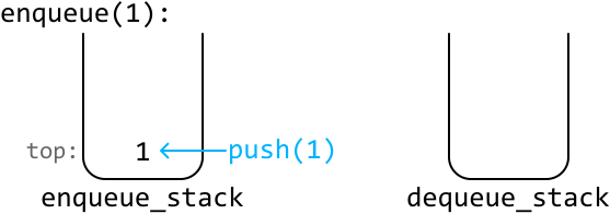
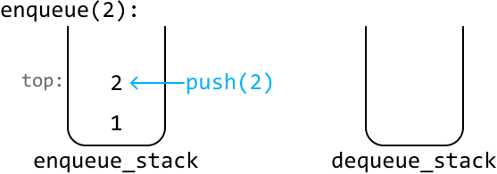
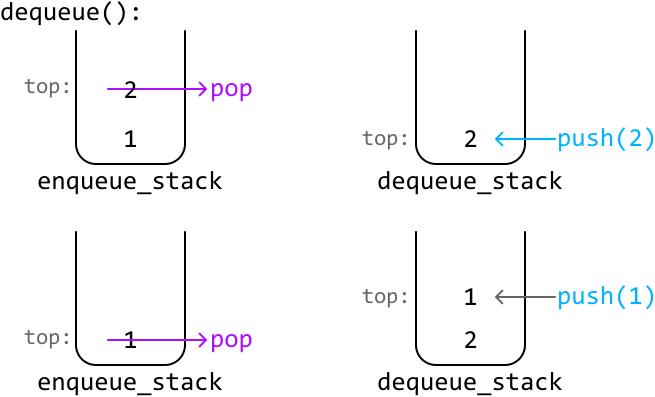
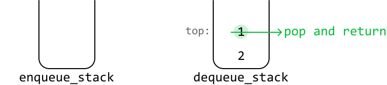
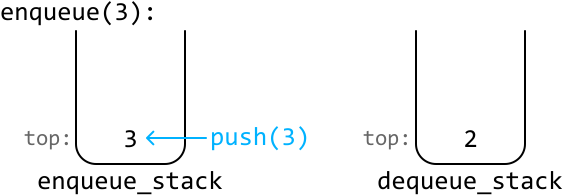
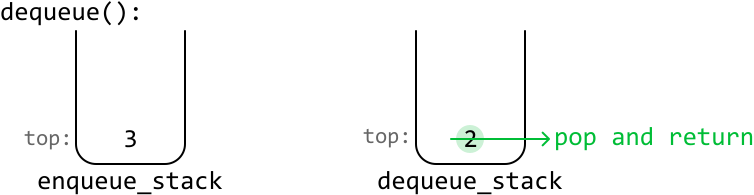
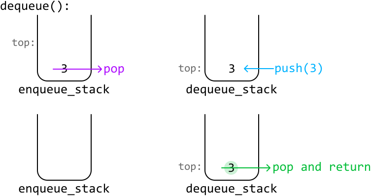
![Image represents a step-by-step illustration of finding the maximum value within an array of integers. Four rows depict the array `[3, 2, 4, 1, 2, 1, 1]`. In each row, a light-blue rectangular highlight progressively moves across the array, indicating the current element being considered as the potential maximum. To the right of each array, 'max = ' is followed by the maximum value found so far during that step. The first three rows show the highlight moving from the leftmost element (3) to the element 4, correctly identifying 4 as the maximum. The final row shows the highlight moving to the last element (1) after 4 has already been identified as the maximum, resulting in a final maximum value of 4. The image visually demonstrates a linear scan algorithm for finding the maximum element in an array.](images/img_fe14e2e1dbd3.svg)
![Image represents two nearly identical arrays of integers, each enclosed in square brackets. The top array is `[3, 2, 4, 1, 2, 1, 1]` and the bottom array is `[3, 2, 4, 1, 2, 1, 1]`. A light-blue rectangular box highlights the sub-array `[2, 4, 1]` in both arrays, indicating that these elements have the same values in both arrays. The text 'same values' is positioned within the central area of the box, explicitly labeling the highlighted section. The arrays are horizontally aligned, with the highlighted sections overlapping vertically. No URLs or parameters are present.](images/img_d8a2fc63d852.svg)
![Image represents a visual depiction of data partitioning or splitting. Two rectangular boxes labeled 'left' and 'right' are positioned above a horizontal array of numbers: [3, 2, 4, 1, 2, 1, 1]. Arrows descend from 'left' and 'right' pointing to the number array. The numbers 3, 2, 4, and 1 are highlighted with a light blue background, indicating that this section of the array is associated with the 'left' box. The remaining numbers (2, 1, 1) are not highlighted and are implicitly associated with the 'right' box. The diagram illustrates how a data set (the array of numbers) is divided into two subsets, 'left' and 'right,' based on some unspecified criteria.](images/img_6e0913b69713.svg)
![Image represents a sliding window algorithm visualization. The initial state shows a numerical array `nums = [2 5 4 3 2 1 3]` where a light-blue rectangle highlights a window encompassing the elements [2 5 4 3 2 1]. A thick grey arrow labeled 'slide window' indicates a rightward shift of this window. The resulting state shows a new window [2 5 4 3 2 1 3] where the element '2' is no longer in the window (indicated by text 'no longer in window' and a downward arrow pointing to the new window), and a new element '3' has entered the window (indicated by text 'new candidate' and a downward arrow pointing to the '3' within the new window). The '3' in the new window is highlighted with a light grey circle to emphasize its addition. The overall diagram illustrates a single iteration of a sliding window technique, showing how the window moves across the array, adding and removing elements.](images/img_8b81840583e1.svg)
![Image represents a step-by-step process demonstrating a coding pattern, likely related to candidate selection or filtering. It begins with an initial list of candidates: `[5 4 3 2 1]`. Step 1, labeled 'remove values ≤ new candidate (3)', shows the removal of values 3, 2, and 1 from the list, resulting in `[5 4]`. A red line visually connects the removed elements. Step 2, 'add the new candidate', inserts the value '3' (in orange) into the list, producing `[5 4 3]`. Finally, step 3, 'remove outdated values', removes the value 5 (indicated by a red line), leaving the final list as `[4 3]`. The process illustrates a sequence of operations involving removing elements based on a condition, adding a new element, and then potentially removing further elements based on another criteria, possibly to maintain a specific list size or order.](images/img_340d390b8b66.svg)
![Image represents a comparison of stack and deque data structures. The left side depicts a stack, labeled 'stack:', showing a linear array represented by `[• • • • • •]`. A cyan-colored arrow labeled 'push' indicates that new elements are added to the right end. Conversely, a purple arrow labeled 'pop' shows that elements are removed from the right end (LIFO - Last In, First Out). The right side illustrates a deque, labeled 'deque:', also represented by a linear array `[• • • • • •]`. However, unlike the stack, the deque has two cyan arrows indicating 'push to left' and 'push to right,' signifying that elements can be added to either end. Similarly, two purple arrows, 'pop from left' and 'pop from right,' demonstrate that elements can be removed from both the left and right ends (FIFO - First In, First Out from one end, and LIFO from the other). The overall image visually contrasts the unidirectional nature of stack operations with the bidirectional capabilities of deque operations.](images/img_9a67178c37c7.svg)
![Image represents a depiction of a queue data structure, showing its initial state and an empty dequeued queue. A numerical array `[3, 2, 4, 1, 2, 1, 1]` is presented, representing the elements of the queue. Beneath each element, a numerical index (0 to 6) indicates its position within the queue. A comma separates the queue array from the representation of the dequeued queue, denoted as `dq = []`, which is an empty array, signifying that no elements have been removed from the original queue yet. The arrangement visually displays the queue's contents and its index-based organization, with the `dq` variable clearly showing the absence of dequeued elements.](images/img_ec8d731fedbd.svg)
![Image represents a visual explanation of a coding pattern, likely involving a deque (double-ended queue) data structure. At the top, two rectangular boxes labeled 'left' and 'right' point downwards with arrows towards an array `[3, 2, 4, 1, 2, 1, 1]`. The number 3 at index 0 is highlighted in light blue, indicating a focus on this element. To the right, two separate, light-grey, dashed-bordered boxes describe operations: the top box states '1) pop candidates ≤ 3', suggesting elements from the array are popped (removed) until a condition (candidates ≤ 3) is met. The bottom box describes '2) push 3 with its index', indicating that the value 3 (and potentially its index 0) is added to another data structure. Finally, an equation `dq = [(3, 0)]` is shown, where `dq` likely represents the deque, and `[(3, 0)]` shows the deque's content after the operations, containing the value 3 paired with its original index 0. The `val` and `index` labels below clarify the tuple's structure within the deque. The entire diagram illustrates a step-by-step process of manipulating an array and updating a deque based on a specific condition.](images/img_5eede20008ec.svg)
![Image represents a visual explanation of a coding pattern, likely involving a deque (double-ended queue) data structure. The top-left shows two labeled boxes, 'left' and 'right,' pointing downwards to an array `[3, 2, 4, 1, 2, 1, 1]`. The numbers 0 through 6 underneath the array represent their indices. The numbers 3 and 2 are highlighted in light blue, indicating they are initial candidates. Two rectangular boxes on the right describe a two-step process: 1) 'pop candidates ≤ 2,' suggesting elements with values less than or equal to 2 are removed from the array; and 2) 'push 2 with its index,' indicating that the value 2 and its index (1) are added to a new data structure. The result of this process is shown as `dq = [(3, 0), (2, 1)]`, where `dq` represents the deque, and each tuple contains a value and its original index from the input array. An arrow labeled 'decreasing values' points to the right, indicating that the deque is ordered by decreasing values.](images/img_5c49e2e90c25.svg)
![Image represents a visual explanation of a coding pattern, likely involving a deque (dq) data structure and a sorting or searching algorithm. The top left shows an array `[3, 2, 4, 1, 2, 1, 1]` with indices 0-6. Arrows labeled 'left' and 'right' point to the elements 3 and 4 respectively, suggesting these are initial boundary points. A dashed box to the right describes a 'pop' operation (step 1) where elements are removed if their value is less than or equal to 4. To the right of this, the deque `dq` is initialized as `[(3, 0), (2, 1)]`, representing value-index pairs. Below, another dashed box describes a 'push' operation (step 2) where the element 4 (at index 2) is added to the deque. The subsequent `dq` becomes `[(4, 2)]`. Red arrows and inequalities (4 > 2, 4 > 3) illustrate comparisons between the current element being considered (4) and elements already in the deque, indicating a process of maintaining a sorted or prioritized subset within the deque. The labels 'val' and 'index' clearly denote the components of each pair within the deque.](images/img_ba43c5265562.svg)
![Image represents a visualization of a coding pattern, likely involving a deque (double-ended queue) data structure. The top-left shows an array `[3, 2, 4, 1, 2, 1, 1]` with a pointer `k` positioned at index 2, indicating a potential split point. Above the array, boxes labeled 'left' and 'right' suggest the array is being processed from both ends. A light-blue highlight spans the array from index 0 to index 3, possibly representing a processed section. The right side displays two labeled boxes describing steps in an algorithm: 1) 'pop candidates ≤ 1' implying elements less than or equal to 1 are removed, and 2) 'push 1 with its index' suggesting that the value 1 and its index are added to a data structure. The result of this algorithm is shown as `dq = [(4, 2), (1, 3)]`, a deque containing pairs where the first element is the value and the second is its original index, arranged in decreasing order of values, as indicated by the arrow labeled 'decreasing values'. The `dq` represents the output after processing the array according to the described steps.](images/img_004ea5a408d5.svg)
![Image represents a visualization of a coding pattern, likely involving a deque (dq) data structure and a sliding window technique. The top-left shows an array `[3, 2, 4, 1, 2, 1]` with indices 0-6. Arrows labeled 'left' and 'right' point to elements 2 and 2 respectively, indicating a window's boundaries. Three numbered, dashed-bordered boxes describe the algorithm's steps: 1) 'pop candidates ≤ 2' which, alongside the right-hand side, shows an initial deque `dq = [(4, 2), (1, 3)]` where each pair represents (value, index) and the element (1,3) is removed because its value is less than or equal to 2; 2) 'push 2 with its index' resulting in `dq = [(4, 2), (2, 4)]`; and 3) 'remove outdated candidates,' which is not explicitly shown in the deque but implies further processing. The right-hand side illustrates the deque's evolution, with a red arrow highlighting the removal of (1,3) and the final deque showing pairs ordered by decreasing values, indicating the algorithm maintains a sorted deque of candidates within the sliding window.](images/img_144ef337a347.svg)
![Image represents a step-by-step illustration of a coding pattern, likely involving a deque (double-ended queue) data structure. The top shows an array `[3, 2, 4, 1, 2, 1]` with indices 0-6. Arrows labeled 'left' and 'right' point to the element '4' and '1' respectively, indicating a focus on a sub-array. Below, three numbered steps describe operations on a deque (`dq`). Step 1) 'pop candidates ≤ 1' suggests removing elements from the deque with values less than or equal to 1. Step 2) 'push 1 with its index' indicates adding the element '1' along with its index (in this case, index 5) to the deque. The result of step 2 is shown as `dq = [(4, 2), (2, 4), (1, 5)]`, where each tuple represents (value, index) pairs, ordered by decreasing values as indicated by the arrow. Finally, step 3) 'remove outdated candidates' implies removing elements from the deque that are no longer relevant based on the algorithm's logic. The entire diagram visualizes the process of maintaining a deque of candidates, ordered by decreasing values, within a specific algorithm.](images/img_34c244847d30.svg)
![Image represents a step-by-step illustration of a coding pattern, likely involving a deque (dq) data structure and a sliding window or similar algorithm. The top shows an array `[3, 2, 4, 1, 2, 1, 1]` with indices 0-6, and arrows pointing from labels 'left' and 'right' to the array's element at index 3 and 6 respectively. Below, three numbered steps are shown, each accompanied by a description and the evolution of the deque `dq`. Step 1, 'pop candidates ≤ 1', shows `dq` initially containing pairs (value, index) representing elements from the array: `[(4, 2), (2, 4), (1, 5)]`. A red arrow indicates the removal of `(1, 5)` because its value (1) meets the condition. Step 2, 'push 1 with its index', adds `(1, 6)` to `dq`, resulting in `[(4, 2), (2, 4), (1, 6)]`. The arrow indicates the deque is ordered by decreasing values. Step 3, 'remove outdated candidates', removes `(4,2)` from `dq` because its index (2) is less than the current `left` pointer (indicated by a red arrow pointing to `(4,2)` and the inequality `2 < left`). The final `dq` is `[(4, 2), (2, 4), (1, 6)]` after this step. The overall process demonstrates how the deque maintains a subset of the array's elements based on value and index, dynamically adapting to the movement of the `left` and `right` pointers.](images/img_1a92c3bb65e2.svg)
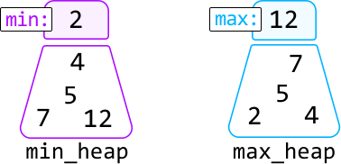
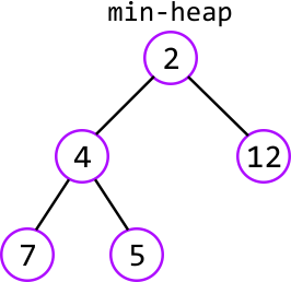
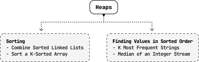
![Image represents a data transformation process where a list of strings is converted into a frequency table. The input is a list `[go coding byte byte go interview go]` containing the strings 'go', 'coding', 'byte', 'byte', 'go', 'interview', and 'go'. This list is shown to the left of a right-pointing arrow. The arrow indicates the flow of data from the input list to the output table. The output is a frequency table labeled 'freqs' with two columns: 'str' representing the unique strings and 'freq' representing their corresponding frequencies. The table lists 'go' with a frequency of 3, 'coding' with 1, 'byte' with 2, and 'interview' with 1. The table visually summarizes the number of occurrences of each unique string from the input list.](images/img_a14144bd52a3.svg)
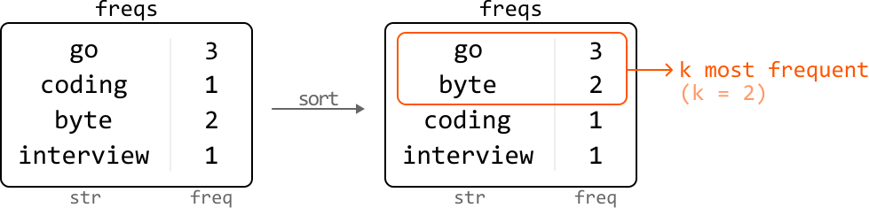
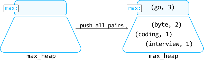
![Image represents a step-by-step visualization of a top-k frequent element algorithm with k=2. The process begins with a max-heap containing three elements: (go, 3), (byte, 2), and (coding, 1). The top element, (go, 3), is identified by a `max:` label and an arrow indicates it's popped from the heap and added to a result list `res`, which initially is empty. This results in a new max-heap containing (byte, 2), (coding, 1), and (interview, 1), and `res` now equals `[go]`. The next iteration identifies (byte, 2) as the maximum, pops it, and adds it to `res`, yielding a max-heap with (coding, 1) and (interview, 1), and `res` becoming `[go, byte]`. The algorithm stops here because k=2, and the final `res` list `[go, byte]` is returned, as indicated by an arrow labeled 'return'. Each max-heap is visually represented as a trapezoid, clearly showing its elements.](images/img_1992cc638876.svg)
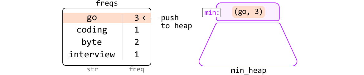
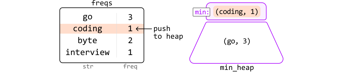
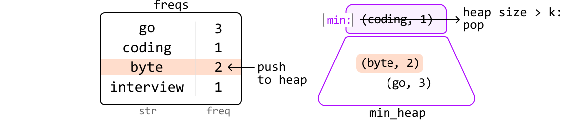
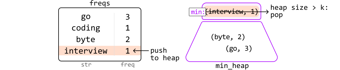
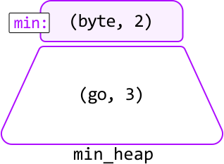
![Image represents a step-by-step visualization of a coding pattern, likely involving a min-heap data structure. The diagram shows three stages. Each stage features a purple, trapezoid-shaped min-heap, labeled 'min_heap,' containing pairs of elements. Above each min-heap is a purple rectangle labeled 'min:' followed by the minimum element currently at the top of the heap. In the first stage, the min-heap contains ('byte', 2) and ('go', 3). A horizontal arrow points from ('byte', 2) to a dashed-line rectangle below labeled 'res = [byte]', indicating that the minimum element ('byte', 2) is popped from the heap and added to a result list 'res'. The second stage shows the min-heap after this operation, containing only ('go', 3). The minimum element ('go', 3) is then popped and added to 'res', resulting in 'res = [byte, go]' in the second dashed-line rectangle. The third stage shows an empty min-heap and the final 'res = [byte, go]' list. A green arrow points from this final 'res' list to the text 'return reverse(res)', indicating that the algorithm concludes by returning the reversed version of the 'res' list.](images/img_fe5d61295b6a.svg)
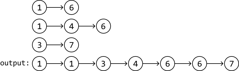




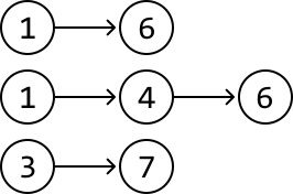
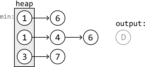
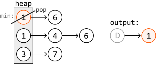
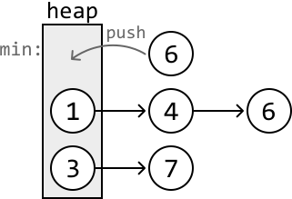
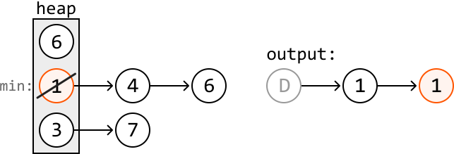
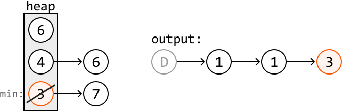
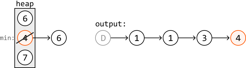
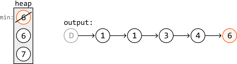



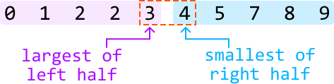

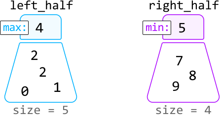
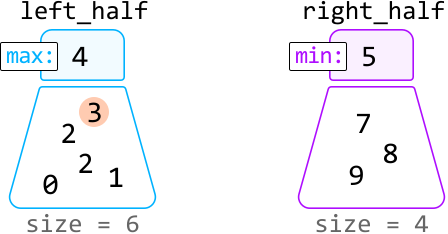
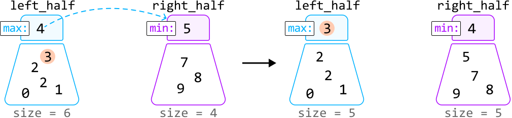
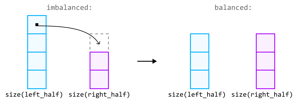
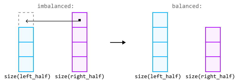
![Image represents a visual depiction of sorting a k-sorted array where k=2. The top row shows the unsorted input array `[5, 1, 9, 4, 7, 10]` with indices 0 through 5 displayed below each element. The bottom row displays the sorted array `[1, 4, 5, 7, 9, 10]` with corresponding indices. Curved arrows connect elements from the unsorted array to their final positions in the sorted array. The arrows illustrate the movement of elements during the sorting process. Specifically, element 5 at index 0 moves to index 2, element 1 at index 1 moves to index 0, element 9 at index 2 moves to index 4, element 4 at index 3 moves to index 1, element 7 at index 4 moves to index 3, and element 10 at index 5 remains at index 5. The gray arrows indicate that the elements are not necessarily directly adjacent in the sorted array, reflecting the k-sorted property (elements are at most k positions away from their sorted position). The text 'k-sorted array:' and 'sorted:' labels the input and output arrays respectively. The value `k = 2` indicates that each element is at most 2 positions away from its correct sorted position in the input array.](images/img_93ab6f49abd3.svg)
![Image represents a visual explanation of a sorting algorithm, likely illustrating a concept related to k-sorted arrays. The diagram shows a k-sorted array `[5, 1, 9, 4, 7, 10]` represented as a trapezoid with a light-blue fill. A horizontal cyan line segment spans the top of the trapezoid, labeled `3 - k` on the left and `3 + k` on the right, indicating a window of size 2k+1 centered around the element at index 3 (assuming 0-based indexing). The number 7 is circled within this window, highlighting its position. The trapezoid's bottom edge connects to a fully sorted array `[1, 4, 5, 7, 9, 10]` below, demonstrating the result of a sorting operation. The number 3 is placed below the sorted array, possibly indicating the index of the middle element in the sorted array or the length of the sorted subarray. The overall structure visually demonstrates how a portion of a k-sorted array (the window) is sorted to obtain a fully sorted array.](images/img_4652cabe212c.svg)
![Image represents a visual explanation of sorting a k-sorted array. The top row shows a 'k-sorted array' [5, 1, 9, 4, 7, 10], labeled as such. A light-blue trapezoid highlights a section of this array, specifically the elements [5, 1, 9]. A horizontal, light-blue arrow above this section points from index θ (zero) to index θ + k, indicating a window of size k elements. The number '1' within the highlighted section is circled, emphasizing its position. The bottom row displays the 'sorted' array [1, 4, 5, 7, 9, 10], resulting from sorting the k-sorted array. A vertical light-blue line connects the beginning of both arrays (index θ), and a diagonal line connects the end of the highlighted section in the k-sorted array to the end of the corresponding sorted section in the sorted array, visually demonstrating the transformation. The diagram illustrates how a portion of a k-sorted array (where each element is at most k positions away from its sorted position) can be sorted to obtain a fully sorted array.](images/img_b067247e335a.svg)
![Image represents a step-by-step illustration of a sorting algorithm applied to a k-sorted array. The top line shows an initial k-sorted array `[5 1 9 4 7 10]`, where a light-blue highlighted sub-array `[5 1 9]` represents a window of size `k` starting at index `0`. A light-blue line extends from index `0` to `0 + k`, indicating the window's boundaries. An arrow points down from a small box containing 'i', suggesting this is the 'i'th iteration of the algorithm. Below, a second line displays the array after a swap operation: `[1 5 9 4 7 10]`. The word 'swapped' and curved arrows indicate that elements 1 and 5 have been swapped. To the right, a dashed box describes the operation performed: 'swap nums[i] with min([5 1 9])', highlighting that the element at index `i` (5) was swapped with the minimum element (1) within the k-sized window. The number 1 is highlighted in peach within the `min()` function to emphasize its selection as the minimum value. The diagram visually demonstrates a single iteration of a sorting algorithm that iteratively swaps elements within a k-sized window to achieve a sorted array.](images/img_3e7ba259d7e9.svg)
![Image represents a step-by-step illustration of a sorting algorithm applied to a k-sorted array. The top section shows the initial k-sorted array `[1 5 9 4 7 10]`, labeled as 'k-sorted array:'. A light-blue rectangle highlights the sub-array [5 9 4] from index 1 (labeled '1' below it) to index 1+k (labeled '1+k' below it). An arrow points down from a box labeled 'i', indicating the index being processed. A dashed box to the right explains the operation: 'swap nums[i] with min([5 9 4])', highlighting '4' as the minimum value within the highlighted sub-array. The bottom section shows the array after the swap, `[1 4 9 5 7 10]`, labeled 'k-sorted array:', with a curved arrow indicating that the elements at indices 1 and 3 have been swapped. The entire diagram visually demonstrates a single iteration of a sorting algorithm (likely a variation of selection sort) on a k-sorted array, focusing on the process of finding and swapping the minimum element within a window of size k.](images/img_49890745e468.svg)
![Image represents a step-by-step illustration of a coding pattern, likely involving a min-heap data structure. The top-left shows an integer variable `k` initialized to 2 and an index variable `i` represented by a box. A downward arrow from `i` points to an array `nums` containing the elements [5, 1, 9, 4, 7, 10], with indices 0 through 5 displayed below each element. To the right, a trapezoidal shape labeled 'min_heap' represents a min-heap data structure with a separate box above it labeled 'min:' indicating the minimum element. A light-gray, dashed-bordered box to the right of the min-heap shows the code snippet `min_heap.push(nums[i])` and `i++`, indicating that the element at index `i` of the `nums` array is being pushed onto the min-heap, and then the index `i` is incremented. The overall diagram visualizes the process of iterating through the `nums` array and adding each element to a min-heap, likely as part of a larger algorithm (e.g., finding the kth smallest element).](images/img_5639fe7cf7de.svg)
![Image represents a step-by-step illustration of building a min-heap from an array. The array `[5, 1, 9, 4, 7, 10]` is shown at the bottom, with indices 0 through 5 labeled below each element. A square box labeled 'i' indicates an index pointer, currently pointing via a downward arrow to the element '1' at index 1. A dashed arrow indicates that the element at index 'i' is being processed. To the right, a trapezoidal shape labeled 'min_heap' represents the min-heap data structure under construction. Currently, it only contains the element '5', labeled with 'min: 5' to its left, indicating it's the minimum value in the heap. A dashed-line box to the right of the min-heap shows the code snippet `min_heap.push(nums[i])` and `i++`, indicating that the element at index `i` (currently 1, the value 1) is being pushed onto the min-heap, and then the index `i` is incremented. The overall diagram visualizes the iterative process of constructing a min-heap by sequentially adding elements from the input array.](images/img_7b5544b29066.svg)
![Image represents a snapshot of a step in an algorithm, likely involving a min-heap data structure. The bottom left shows an array `nums` = [5, 1, 9, 4, 7, 10] with indices 0 through 5 displayed below each element. A box labeled 'i' points via a dashed arrow to the element 9 at index 2, indicating the current iteration of a loop. To the right, a purple trapezoid labeled 'min_heap' visually represents a min-heap containing the value 5 at its root and 1 at the top. A separate purple box labeled 'min:' displays the value 1, representing the minimum element currently in the min-heap. A dashed-line box to the right of the min-heap shows the code snippet `min_heap.push(nums[i])` followed by `i++`, indicating that the algorithm is pushing the element at index `i` (which is 9) onto the min-heap and then incrementing `i` for the next iteration. The overall diagram illustrates the process of building a min-heap from an array by iteratively pushing elements onto the heap.](images/img_994998ad4ddf.svg)
![Image represents a visual depiction of a step in a sorting algorithm, likely using a min-heap data structure. The left side shows an array `[5, 1, 9, 4, 7, 10]` indexed from 0 to 5, with a pointer `i` currently at index 3, indicating the element '4'. A dashed arrow points from `i` to '4', suggesting that element '4' is being considered or processed. Below the array is a labeled axis 'k + 1', implying 'k' represents a variable related to the algorithm's progress. The right side displays a min-heap, a tree-based data structure where the smallest element is at the root. The min-heap contains the elements 1, 5, and 9, with '1' at the top, labeled 'min: 1', indicating it's the minimum value in the heap. The overall image suggests that the algorithm is building or updating the min-heap by incorporating elements from the array, with the current focus on element '4' at index 3.](images/img_eb8f19d183a9.svg)
![The image represents a step in a sorting algorithm, likely using a min-heap data structure. On the left, a numbered array `[5, 1, 9, 4, 7, 10]` is shown, with indices 0 through 5 displayed below. A box labeled 'insert_index' points down to this array, indicating a position where a value will be inserted. Separately, a box labeled 'i' points to the same array, likely representing an iterator or index variable. To the right, a min-heap is depicted as a triangular structure containing the values 5 and 9. Above the min-heap, a purple box labeled 'min:' contains the value '1,' representing the minimum element currently in the heap. An arrow connects this '1' to a dashed box containing the code snippet `nums[insert_index] = min_heap.pop()`. This code signifies that the minimum value (1) from the `min_heap` is being popped (removed) and assigned to the array element at the index specified by `insert_index`. The overall diagram illustrates the process of inserting a value into a sorted array using a min-heap to efficiently find the smallest element.](images/img_74e8425bca21.svg)
![Image represents a step-by-step illustration of building a min-heap from an array. The top half shows the initial state: an array `[1, 1, 9, 4, 7, 10]` is depicted with indices 0-5 below each element. A variable `insert_index` points to the first element (index 0), and a variable `i` points to the element at index 3 (value 4). A partially-filled min-heap is shown to the right, containing only the value 9, with a label `min: 5` indicating the minimum value (5) which is not yet in the heap. A dashed box next to the min-heap displays the code snippet `min_heap.push(nums[i])`, `insert_index++`, `i++`, indicating that the element at index `i` (4) is being pushed onto the min-heap, `insert_index` is incremented, and `i` is incremented. The bottom half shows the next step: `insert_index` now points to the element at index 3 (value 4), and `i` points to the element at index 4 (value 7). The min-heap now contains 4, 5, and 9, with `min: 4` indicating the current minimum. Dashed arrows indicate the movement of `insert_index` and `i` through the array. The overall diagram visualizes the iterative process of constructing a min-heap by sequentially adding elements from an array.](images/img_bbed6962032d.svg)
![Image represents a step-by-step illustration of a sorting algorithm, likely using a min-heap data structure. The top half shows an initial state: an array `nums` containing `[1, 1, 9, 4, 7, 10]` is indexed by `insert_index` (initially pointing to the first element, highlighted in green) and `i` (pointing to the second element). A min-heap, labeled `min_heap`, contains the values `5` and `9`. An arrow indicates that the minimum value from the min-heap (4, highlighted in purple) is assigned to `nums[insert_index]`, replacing the initial value. The bottom half depicts the next step: `insert_index` has advanced to the next position. The value at `nums[i]` (4) is pushed onto the `min_heap`, updating it to contain `5` and `9`. A separate box describes the actions performed: popping the minimum element from the min-heap and assigning it to the array element at `insert_index`, then pushing the next array element onto the min-heap, incrementing both `insert_index` and `i`. The array and min-heap are visually represented, showing the changes in their contents after each step.](images/img_70dba6c87cd4.svg)
![Image represents a visual explanation of a coding pattern, likely involving a min-heap data structure and an array. The top half shows an array `nums` represented as `[1, 4, 9, 4, 7, 10]` with indices 0-5, and a min-heap `min_heap` containing the values 7 and 9. A box labeled 'insert_index' points to the element '9' in the array. A purple box labeled 'min: 5' indicates the minimum value (5) is being extracted from the min-heap. An arrow connects this to a dashed box showing the operation `nums[insert_index] = min_heap.pop()`, which replaces the element at `insert_index` (9) with the minimum value from the heap (5). The bottom half shows the result of this operation: the array is now `[1, 4, 5, 4, 7, 10]`, and the min-heap contains only 9. A box labeled 'i' points to the next element (7) in the array. A dashed box shows the operation `min_heap.push(nums[i])`, `insert_index++`, `i++`, indicating that the next element (7) is pushed onto the min-heap, and the `insert_index` and `i` are incremented. The overall diagram illustrates a step-by-step process of replacing array elements with values from a min-heap, likely part of a sorting or selection algorithm.](images/img_dc4bbc1cdf9f.svg)
![Image represents a visual depiction of inserting an element into a min-heap data structure. The left side shows an array `[1, 4, 5, 4, 7, 10]` with indices 0 through 5 displayed below. A box labeled 'insert_index' points via a dashed arrow to the element '4' at index 3, indicating where a new element is to be inserted. On the right, a min-heap is shown, represented as a trapezoidal structure with elements 7 (labeled 'min: 7' in a box), 9, and 10. A box labeled 'i' points via a dashed arrow to the element '10' in the array, suggesting the index from which the element is being inserted into the heap. The array and the min-heap are visually separate but conceptually linked, illustrating the process of adding an element to the heap, which would involve comparing and potentially swapping elements to maintain the min-heap property.](images/img_cc57144035d7.svg)
![Image represents a step in a sorting algorithm, likely using a min-heap data structure. The algorithm involves an array `nums` represented by `[1, 4, 5, 4, 7, 10]` with indices shown below. A separate min-heap, `min_heap`, is depicted as a trapezoidal structure containing the values 9 and 10. A variable `insert_index` points to the next available position in `nums` (index 3 in this case). A purple box labeled `min: 7` represents the minimum value currently in the `min_heap`. A rightward arrow connects this box to a dashed box containing the code snippet `nums[insert_index] = min_heap.pop(); insert_index++;`. This code indicates that the minimum element (7) from the `min_heap` is being popped and assigned to the element at `nums[insert_index]`, after which `insert_index` is incremented. The overall process illustrates how the algorithm uses the min-heap to efficiently find and place the next smallest element into its correct sorted position within the `nums` array.](images/img_e267df1a879a.svg)
![Image represents a step in a sorting algorithm, likely heapsort, illustrating the process of inserting elements from a list into a min-heap. A numbered list `[1, 4, 5, 7, 7, 10]` is shown, with indices 0-5 displayed below. A variable `insert_index` points to the next available position (index 3) in the list. A purple min-heap is depicted, currently containing only the value 10. A separate purple box labeled `min: 9` represents the minimum value extracted from the min-heap. A dashed-line box contains the code snippet `nums[insert_index] = min_heap.pop(); insert_index++;`, indicating that the minimum element (9) from the `min_heap` is being assigned to the element at `insert_index` in the `nums` array, and then `insert_index` is incremented. An arrow connects the `min: 9` box to the code snippet, showing the data flow. The algorithm appears to be iteratively removing the minimum element from the min-heap and placing it into its correct sorted position within the `nums` array.](images/img_c452ce4eccc3.svg)
![Image represents a step in a sorting algorithm, likely using a min-heap data structure. The left side shows an array `nums` with elements [1, 4, 5, 7, 9, 10] indexed from 0 to 5. A box labeled 'insert_index' points to the element '10' at index 5, indicating the current position for insertion. A purple box labeled 'min: 10' represents the minimum element (10) extracted from a min-heap data structure depicted as a purple trapezoid labeled 'min_heap'. A right-pointing arrow connects the 'min: 10' box to a grey box containing the code snippet `nums[insert_index] = min_heap.pop(); insert_index++;`. This code signifies that the minimum value (10) from the min_heap is assigned to the array element at `insert_index`, and then `insert_index` is incremented, preparing for the next element insertion. The overall process illustrates how a sorted array is constructed by repeatedly extracting the minimum element from a min-heap and placing it into its correct position in the array.](images/img_6c763a81889d.svg)
![Image represents a visual depiction of a min-heap data structure. On the left, a green array `[1, 4, 5, 7, 9, 10]` is shown, with indices 0 through 5 displayed below each element. To the right, a trapezoidal shape labeled 'min_heap' represents the heap structure itself. Above the heap, a small purple rectangle labeled 'min:' suggests this area displays the minimum value within the heap (which would be 1 in this case, based on the array). There's no explicit connection drawn between the array and the heap, but the implication is that the array's elements are stored in the min-heap according to the min-heap property (where the parent node is always less than or equal to its children).](images/img_07e2330bb295.svg)




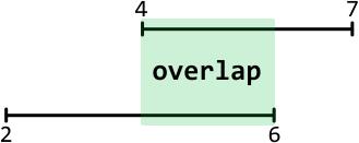
![Image represents a data structure illustrating the concept of intervals. The top line defines a list named `intervals` containing five sub-lists, each representing an interval. These sub-lists are `[1, 6]`, `[2, 4]`, `[5, 9]`, `[8, 10]`, and `[10, 12]`. The second line shows a list called `start points` containing the start values of each interval, extracted from the `intervals` list: `[1, 2, 5, 8, 10]`. These values are highlighted in cyan. The third line displays a list named `end points`, which contains the corresponding end values of each interval from the `intervals` list: `[4, 6, 9, 10, 12]`. These values are highlighted in orange. The arrangement visually demonstrates how the `start points` and `end points` lists are derived from the `intervals` list, showing a clear relationship between the intervals and their constituent start and end points.](images/img_c26623ff495d.svg)
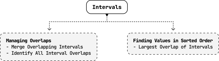
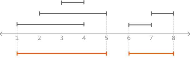
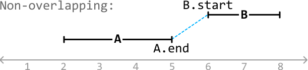
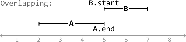
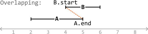
![Image represents a sequence of five distinct arrays, each enclosed in square brackets `[]` and containing two integer elements separated by a comma `,`. The arrays are arranged horizontally, adjacent to one another without any intervening spaces. The first array contains the integers 3 and 4; the second, 7 and 8; the third, 2 and 5; the fourth, 6 and 7; and the fifth, 1 and 4. No information flows between the arrays; they are presented as independent data structures. There are no URLs or parameters present.](images/img_e715c82f0bb2.svg)
![Image represents a diagram illustrating a sorting operation on a list of sub-lists. The top row shows five sub-lists, each containing two numbers: [3, 4], [7, 8], [2, 5], [6, 7], and [1, 4]. A downward-pointing arrow labeled 'sort' connects the top and bottom rows. The bottom row displays the same five sub-lists, but now each sub-list is sorted in ascending order: [1, 4], [2, 5], [3, 4], [6, 7], and [7, 8]. The diagram visually demonstrates the application of a sorting algorithm to each individual sub-list, leaving the order of the sub-lists themselves unchanged.](images/img_0d9f93a6d169.svg)

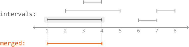

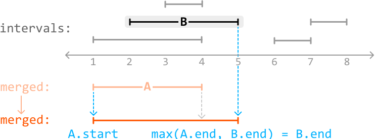

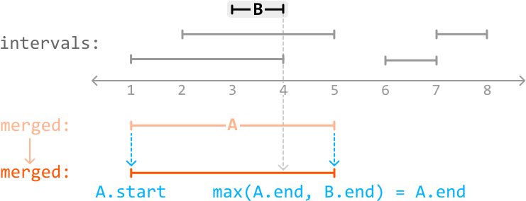

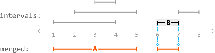

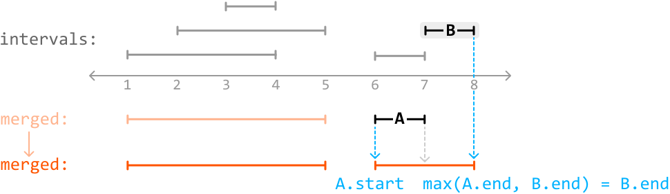


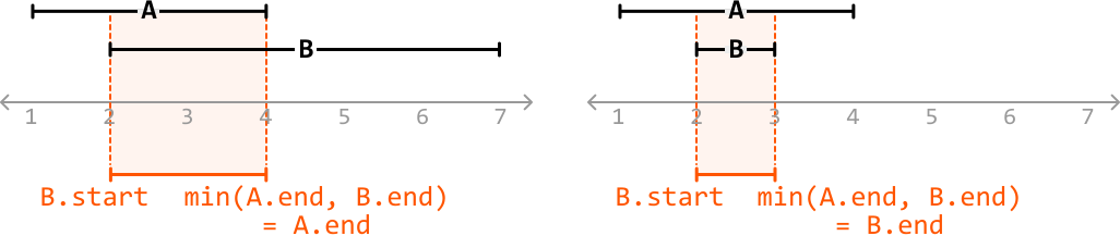



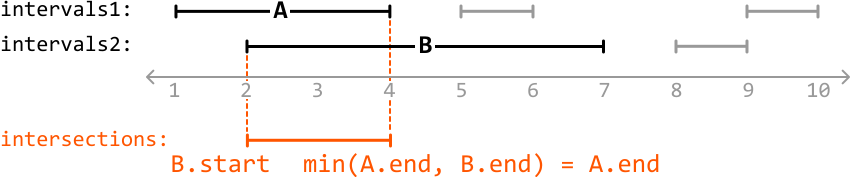

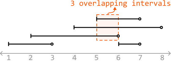
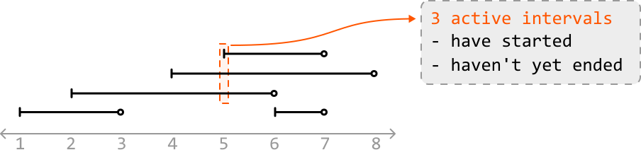



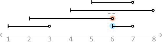


![Image represents a coding pattern illustration demonstrating the transformation of a list of intervals into a sorted list of points. The top line shows a Python-like list called `intervals` containing five sub-lists, each representing an interval with a start and end point: `[1, 3]`, `[2, 6]`, `[4, 8]`, `[6, 7]`, and `[5, 7]`. A right arrow indicates a transformation to the `points` list below, which contains all the start and end points from the `intervals` list: `[1 2 3 4 5 6 6 7 7 8]`. Underneath each point in the `points` list, 'S' (in light blue) denotes a start point of an interval and 'E' (in orange) denotes an end point. A small downward-pointing arrow underlines the 'E' and 'S' representing an end point appearing before a start point, highlighting a condition where the end point of one interval is sorted before the start point of another. The text 'end point sorted before start point' explains this specific arrangement and the implication of the sorting process.](images/img_9cb1046aa638.svg)
![Image represents a Python-like list assignment. The variable `spendings` is assigned a list containing five integer values: `10`, `15`, `20`, `10`, and `5`. These values are enclosed within square brackets `[]`, indicating a list data structure. Below the list, the days of the week—Monday (Mon), Tuesday (Tue), Wednesday (Wed), Thursday (Thu), and Friday (Fri)—are aligned with the corresponding numerical values in the list, implying that each number represents the spending for that particular day. The overall structure shows a simple data representation where daily spending is stored in a list, with the list's index implicitly representing the day of the week.](images/img_7e353059f0f4.svg)
![Image represents a comparison of two arrays: 'spendings' and 'prefix_sums'. The 'spendings' array, shown as `spendings = [10 15 20 10 5]`, lists daily spending amounts for Monday through Friday, respectively. Each spending value is aligned vertically with its corresponding day label (Mon, Tue, Wed, Thu, Fri) in a lighter gray font. Below this, the 'prefix_sums' array, displayed as `prefix_sums = [10 25 45 55 60]`, shows the cumulative sum of spending up to and including each day. For example, the first element (10) is the spending for Monday, the second element (25) is the sum of Monday's and Tuesday's spending (10 + 15), the third (45) is the sum of Monday, Tuesday, and Wednesday's spending (10 + 15 + 20), and so on. The arrangement clearly demonstrates the relationship between daily spending and its running total, illustrating the concept of prefix sums.](images/img_a1aee8b03347.svg)
![Image represents a step-by-step calculation of prefix sums for an array. The top row shows the input array `[10, 15, 20, 10, 5]`. Each element in this array is represented by a vertical orange line pointing downwards. The label 'prefix_sums = [10' indicates the initialization of a new array to store the prefix sums. Subsequent rows show the iterative calculation. Each orange line represents the addition of the current element to the running sum. Curved peach arrows indicate the addition operation (+), connecting the previous prefix sum to the current element. The resulting prefix sums are shown in each row within square brackets: `[10]`, `[10, 25]`, `[10, 25, 45]`, `[10, 25, 45, 55]`, and finally `[10, 25, 45, 55, 60]`. The process demonstrates how each element in the prefix sums array is the cumulative sum of all preceding elements in the input array.](images/img_3670261d176d.svg)
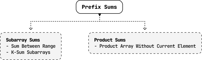
![Image represents three examples of a `sum_range` function operating on a numerical array `[3, -7, 6, 0, -2, 5]`. Each example shows the array with indices 0-5 displayed below each element. The function `sum_range(start_index, end_index)` calculates the sum of elements within a specified range (inclusive). The first example, `sum_range(0, 3)`, highlights elements at indices 0, 1, 2, and 3 (3, -7, 6, 0) in a light-blue box, with a blue arrow above indicating their sum, `sum = 2`. The second example, `sum_range(2, 4)`, highlights elements at indices 2, 3, and 4 (6, 0, -2), showing `sum = 4` above the highlighted section. Finally, `sum_range(2, 2)` highlights only the element at index 2 (6), resulting in `sum = 6`. In all cases, the function's parameters (start and end indices) are clearly visible, along with the resulting sum displayed above the highlighted portion of the array.](images/img_0ccbefe610b0.svg)
![Image represents a code snippet illustrating the concept of prefix sum. The top line declares a Python list named `nums` containing the integer values [3, -7, 6, 0, -2, 5]. Below this, faint gray numbers [0, 1, 2, 3, 4, 5] are shown as indices for the `nums` list. The second line declares another list named `prefix_sum`. This list contains the prefix sums of the `nums` list. `prefix_sum`'s values are calculated cumulatively: the first element is the same as the first element in `nums` (3), the second is the sum of the first two elements of `nums` (3 + (-7) = -4), the third is the sum of the first three (3 + (-7) + 6 = 2), and so on. Similarly, faint gray numbers [0, 1, 2, 3, 4, 5] are shown as indices for the `prefix_sum` list, aligning with the corresponding elements in `nums`. The arrangement visually demonstrates the relationship between an original list and its prefix sum, showing how each element in `prefix_sum` is the cumulative sum of the preceding elements in `nums`.](images/img_7d7f16c67591.svg)
![Image represents a visual explanation of prefix sum calculation. The top line shows the equation `sum_range(0, 3) = prefix_sum[3]`, indicating that the sum of elements from index 0 to 3 in an array is equal to the value at index 3 in the prefix sum array. Below, an array named `nums` is shown with values [3, -7, 6, 0, -2, 5], with indices 0 through 5 displayed beneath each element. A light-blue background highlights elements at indices 0, 1, 2, and 3. A cyan-colored line segment above the highlighted portion indicates the range of summation, labeled 'sum = 2,' representing the sum of the highlighted elements (3 + (-7) + 6 + 0 = 2). A downward arrow points from the highlighted section of `nums` to an array named `prefix_sum`. `prefix_sum` contains the cumulative sums of `nums`; its values are [3, -4, 2, 2, 0, 5], with indices 0 through 5 displayed beneath each element. The value at index 3 in `prefix_sum` (2) matches the calculated sum of `nums` from indices 0 to 3, visually demonstrating the prefix sum concept.](images/img_1fc594807732.svg)
![Image represents a visual depiction of a sub-array within a larger array. The larger array is shown partially, with elements `[3, -7]` on the left and `[5]` on the right. These elements are vertically stacked with their indices shown in grey below: `0` and `1` under `[3, -7]` and `5` under `[5]`. The central portion of the image highlights a sub-array `[6, 0, -2]` in a light blue background. This sub-array's indices are also shown in grey below, indicating positions `2`, `3`, and `4` respectively. The arrangement visually demonstrates how a sub-array is a contiguous section of a larger array, selected by its starting and ending indices. The indices are used to access specific elements within the array.](images/img_f72141273bdd.svg)
![Image represents a visual depiction of a sub-array within a larger array. A light-blue rectangular area displays a numerical array [3, -7, 6, 0, -2], with indices [0, 1, 2, 3, 4] shown faintly below each element. Above this array, a bright-blue line segment extends horizontally, marked with small perpendicular lines at its ends. A small triangle points downwards from the line segment, positioned above the element '0' at index 3. The text 'sum[0 : 4]' is written in blue above the line, indicating that a sum is being calculated from index 0 up to (but not including) index 4. The number '5' is shown outside the light-blue rectangle to the right, likely representing an element beyond the sub-array being considered. The overall image illustrates a sub-array selection and a potential summation operation within a larger array context.](images/img_0c979c16069d.svg)
![Image represents a visual depiction of array summation. A numerical array `[3, -7, 6, 0, -2, 5]` is shown, partitioned into sub-arrays. The first two elements, `[3, -7]`, are highlighted in light gray with red diagonal lines, and a red line segment below indicates their summation, labeled `sum[0: 1]`. The next three elements, `[6, 0, -2]`, are highlighted in light blue, with a light blue line segment below indicating their summation, labeled `sum[2: 4]`. A light blue line segment above encompasses the entire array from index 0 to 4, representing the total sum of the array, labeled `sum[0: 4]`. The element at index 5, `5`, is shown separately, not included in any summation. The indices of each element are subtly indicated below the numbers within the array.](images/img_bf78146bf002.svg)
![Image represents three identical arrays, each enclosed in square brackets `[]`, containing the integer sequence `[1, 2, -1, 1, 2]`. Each array is displayed horizontally, with the elements numbered underneath from 0 to 4, representing their indices. A peach-colored rectangular highlight spans the first three elements (1, 2, -1) in each array. Above each array, the text 'sum = 3' is displayed in orange, indicating that the sum of the highlighted elements (1 + 2 + (-1) = 3) within the peach-colored region equals 3. The arrangement visually emphasizes the consistent sub-array and its sum across the three repetitions.](images/img_4e1071cdbf32.svg)
![Image represents a visual explanation of calculating a subarray sum using prefix sums. The image shows three arrays. The first array `[1 2 -1 1 2]` is the input array. Above it, in orange text, is labeled `sum[i:j]`, representing the sum of a subarray from index `i` to `j`. A peach-colored rectangle highlights the subarray `[-1 1]` which is the sum of elements from index `i` to `j`. Arrows point from small boxes labeled `i` and `j` upwards to the elements at those indices within the subarray. The second array `[1 2 -1 1 2]` is labeled `prefix_sum[j]` in light blue text, representing the prefix sum array up to index `j`. A light blue rectangle highlights the prefix sum up to `j`, which is `[1 2 -1 1]`. An arrow points from a box labeled `j` to the last element of this prefix sum. The third array `[1 2 -1 1 2]` is labeled `prefix_sum[i - 1]` in red text, representing the prefix sum up to index `i - 1`. A light pink rectangle highlights the prefix sum up to `i-1`, which is `[1 2]`. An arrow points from a box labeled `i - 1` to the last element of this prefix sum. The equation `[1 2 -1 1 2] = [1 2 -1 1 2] - [1 2]` demonstrates that the subarray sum `sum[i:j]` can be calculated by subtracting the prefix sum up to `i - 1` from the prefix sum up to `j`.](images/img_56a33d29e0e5.svg)
![Image represents a visual explanation of prefix sum calculation. The image shows two arrays: a peach-colored array labeled `sum[0: j]` containing the elements [1, 2, -1, 1, 2], and a light-blue array labeled `prefix_sum[j]` containing [1, 2, -1, 1, 2]. Both arrays contain the same numerical values. An upward arrow connects the index `j` (represented by a small gray square) to both arrays, indicating that `j` is the index up to which the sum is calculated. The `sum[0: j]` array represents a sub-array from index 0 up to index `j` of the original array, while the `prefix_sum[j]` array represents the cumulative sum of the elements from index 0 up to index `j`. The equality sign (=) between the arrays visually demonstrates that the `prefix_sum[j]` array is the result of calculating the cumulative sum of the `sum[0: j]` array. The subscript `0` in `sum[0: j]` indicates that the summation starts from the beginning of the array.](images/img_b8d9236ee7c9.svg)
![Image represents a visual explanation of prefix sums. The top line shows an array named `nums` containing the integer values [1, 2, -1, 1, 2]. Below it, an array named `prefix_sums` is shown, containing the cumulative sums of `nums`. `prefix_sums` starts with 1 (the first element of `nums`), then adds the second element (2) to get 3, then adds the third element (-1) to get 2, and so on, resulting in the array [1, 3, 2, 3, 5]. An orange arrow labeled 'start prefix sums with 0' points downwards from above to the beginning of a third array, visually demonstrating that a prefix sum calculation often begins with 0. This third array is identical to `prefix_sums` except it includes a leading 0, representing the cumulative sum before considering any elements from `nums`. The indices of each array are shown below the arrays for clarity.](images/img_69a36c54587d.svg)
![Image represents a visual depiction of a prefix sum calculation and its mapping. The image shows an integer array `[1, 2, -1, 1, 2]` labeled with indices 0 through 4 beneath each element. Above the array, `k = 3` is specified, indicating a parameter likely related to a window or sub-array size. To the right, a table labeled 'prefix_sum_map' is presented. This table has two columns: 'sum' and 'freq'. The 'sum' column contains the value `0`, representing the initial prefix sum. The 'freq' column contains the value `1`, indicating the frequency of this sum. The arrangement suggests that the array is processed to calculate prefix sums, and the `prefix_sum_map` stores the unique prefix sums encountered and their frequencies. The value of `k` likely influences how these prefix sums are calculated or used in a larger algorithm, possibly defining a sliding window of size 3 across the input array.](images/img_cd74270b349a.svg)
![Image represents a step-by-step illustration of a coding pattern, likely related to prefix sums or subarray sums. The top left shows `k = 3` indicating a parameter value. Below, `curr_prefix_sum = 1` represents the current prefix sum, which is an arrow pointing down to an array `[1, 2, -1, 1, 2]` indexed from 0 to 4. To the right, a `prefix_sum_map` is shown as a table with two columns labeled `sum` and `freq`, currently containing only one row with `sum = 0` and `freq = 1`. A dashed box to the right shows a conditional statement: `curr_prefix_sum - k = -2 (not in hash map) => continue`. This indicates that the difference between the current prefix sum (1) and k (3) is -2, which is not found as a `sum` in the `prefix_sum_map`, resulting in the continuation of the algorithm. The overall diagram depicts a single iteration of an algorithm that likely involves tracking prefix sums and checking for specific sum values within a hash map (or similar data structure) to solve a problem, possibly related to finding subarrays with a given sum.](images/img_ea33c3360c21.svg)
![Image represents a visual explanation of a coding pattern, likely related to prefix sums and hash maps. The top-left shows 'k = 3' indicating a parameter value. Below, 'curr_prefix_sum = 3' suggests a running prefix sum. An array `[1, 2, -1, 1, 2]` is displayed with indices 0-4 beneath, illustrating the data being processed. A downward arrow connects 'curr_prefix_sum = 3' to the array, implying the sum is derived from the array elements. To the right, a 'prefix_sum_map' is depicted as a table with two columns labeled 'sum' and 'freq'. This table contains two rows: one with 'sum' = 0 and 'freq' = 1, and another with 'sum' = 1 and 'freq' = 1, representing prefix sums and their frequencies. A light-grey box on the far right details a calculation: 'curr_prefix_sum - k = 0 (in hash map)' which implies checking if a specific prefix sum exists in the map. The subsequent line 'count += prefix_sum_map[0] += 1' shows an increment to a 'count' variable based on the frequency found in the 'prefix_sum_map' at index 0. The arrow connecting the 'prefix_sum_map' and the calculation box indicates data flow from the map to the calculation. The entire diagram illustrates a step-by-step process of using prefix sums and a hash map to efficiently solve a problem, likely counting subarray sums equal to a target value (k).](images/img_691df9292167.svg)
![Image represents a visualization of a coding pattern, likely for finding subarrays with a specific sum. The top-left shows 'k = 3', indicating a target sum. Next to it, 'curr_prefix_sum = 2' represents the current prefix sum calculated so far. An array [1, 2, -1, 1, 2] is shown below, with indices 0 to 4 displayed beneath each element. A downward arrow connects 'curr_prefix_sum = 2' to the '-1' element in the array, indicating the current prefix sum calculation stage. To the right is a table labeled 'prefix_sum_map', showing prefix sums (3, 1, 0) in the left column and their frequencies (1, 1, 1) in the right column. Finally, a light-gray box on the far right displays 'curr_prefix_sum - k = -1 (not in hash map)' and an arrow pointing right labeled 'continue', suggesting that if the difference between the current prefix sum and the target sum (k) is not found in the 'prefix_sum_map', the algorithm continues processing the array.](images/img_525bcfd90def.svg)
![Image represents a visual explanation of a coding pattern, likely for finding subarrays with a sum equal to a target value (k=3 in this case). The left side shows an input array `[1, 2, -1, 1, 2]` with indices displayed below. Above it, `curr_prefix_sum = 3` indicates a running prefix sum at a particular point. A downward arrow points to the element '1' at index 3, suggesting this is the current prefix sum being considered. To the right, a table labeled `prefix_sum_map` stores prefix sums (in the 'sum' column) and their frequencies (in the 'freq' column). For example, a prefix sum of 0 has a frequency of 1, a prefix sum of 1 has a frequency of 1, a prefix sum of 2 has a frequency of 1, and a prefix sum of 3 has a frequency of 1. A light peach-colored cell highlights the prefix sum of 0 and its frequency of 1. A dashed-line box on the far right describes the algorithm's logic: if `curr_prefix_sum - k == 0`, meaning the current prefix sum minus the target sum is zero, then increment a `count` variable by the frequency of that prefix sum found in `prefix_sum_map` at index 0 (which is 1 in this case). The `+= 1` indicates that the count is incremented by 1. The entire diagram illustrates how a prefix sum map is used to efficiently count subarrays with a specific sum.](images/img_b86b27199343.svg)
![Image represents a visual explanation of a coding pattern, likely for finding subarrays with a sum equal to a target value (k=3 in this case). The left side shows an input array `[1, 2, -1, 1, 2]` with indices displayed below. Above it, `curr_prefix_sum = 5` indicates the cumulative sum of the array. A downward arrow points to the array, suggesting this sum is being processed. The center displays a `prefix_sum_map`, a table with two columns: 'sum' and 'freq' (frequency). This table stores prefix sums and their counts. The cell (2,1) is highlighted in peach, indicating a prefix sum of 2 has occurred once. The right side shows a calculation step: `curr_prefix_sum - k = 2` (where k=3), implying a search for subarrays summing to 3. The result, 2, is used to access the `prefix_sum_map[2]`, which is 1 (the frequency of prefix sum 2). This value (1) is then added to a `count` variable (`count += 1`), suggesting the algorithm is counting occurrences of subarrays with the target sum. The entire diagram illustrates how a prefix sum map is used to efficiently count subarrays with a given sum.](images/img_bf76aecfbcf0.svg)
![Image represents a calculation demonstrating a coding pattern. The left side shows an array `[2, 3, 1, 4, 5]` with each element visually connected via orange curved lines to a central node labeled 'product = 120'. This indicates that the product of all elements in the array is 120. An arrow points to the right, leading to a calculation where 120 is divided by each element of the original array: `res = [120/2, 120/3, 120/1, 120/4, 120/5]`. Below this, the results of these divisions are shown as a new array: `res = [60, 40, 120, 30, 24]`. The diagram visually illustrates the process of calculating the result of dividing a product by each of its factors.](images/img_84e515f43f52.svg)
![Image represents a diagram illustrating a coding pattern, likely related to array processing or a similar data structure. A top-level element labeled 'i' points downwards to an array-like structure visually divided into two parts. The left part, highlighted in light blue, contains the numbers '2' and '3', with a calculation 'product = 6' indicating their multiplication. The right part, highlighted in light purple, contains '4' and '5', with a corresponding calculation 'product = 20'. A gray brace connects the results of these sub-calculations ('6' and '20'), leading to a final calculation 'res[i] = 6 * 20 = 120', showing the multiplication of the two sub-products and assigning the result (120) to an array element 'res[i]', where 'i' likely represents an index. The diagram visually demonstrates a process where sub-arrays are processed independently to produce intermediate results, which are then combined to generate a final result.](images/img_786a6714a8ab.svg)
![Image represents a step-by-step calculation of the product of all elements in an array except the element at the current index. The top row shows an input array `nums` containing the integers [2, 3, 1, 4, 5]. Below this, `left_products` array stores the cumulative product of elements to the left of each index in `nums`, starting with 1 (the product of zero elements). Each element in `left_products` is calculated by multiplying the previous element by the corresponding element in `nums`. Similarly, `right_products` calculates the cumulative product of elements to the right of each index, starting from the rightmost element and moving left. Asterisks (*) visually represent the multiplication operations between consecutive elements in `nums` to obtain `left_products`. Double vertical lines (||) represent the multiplication between corresponding elements of `left_products` and `right_products` to produce the final `res` array, which contains the product of all elements in `nums` except the element at the current index. For example, `res[0]` (60) is calculated as `left_products[0]` (1) * `right_products[0]` (60).](images/img_dc50ee8eea98.svg)
![Image represents a code snippet showcasing an array named `nums` initialized with the integer values [2, 3, 1, 4, 5]. Below it, another array named `left_products` is partially shown, initialized with the value `[1` suggesting it's an array intended to store the product of numbers to the left of each element in the `nums` array. The arrangement is vertical, with `nums` above `left_products`, implying a sequential relationship where `left_products` is likely calculated based on the values in `nums`. No explicit connections or information flow are visually depicted beyond the implied relationship between the two arrays; the image only shows the initial state of the arrays before any computation is performed. There are no URLs or parameters present.](images/img_2d97a469816f.svg)
![Image represents a visual depiction of a calculation step within a coding pattern, likely related to prefix or suffix product calculation. The top line shows a list named 'nums' containing the integer array [2, 3, 1, 4, 5]. Below, a list named 'left_products' is initialized as an array. Gray arrows indicate that the initial values of 'nums' (2 and then 3) are being processed. A central asterisk (*) symbolizes a calculation operation. An orange arrow shows the result of this operation (2, likely the product of 2 and 1) being appended to 'left_products'. The diagram suggests an iterative process where elements from 'nums' are sequentially multiplied and accumulated into 'left_products', representing a running product from the left side of the 'nums' array. The incomplete 'left_products' array and the continuation of 'nums' imply that the calculation is ongoing.](images/img_bc830b52e9b2.svg)
![Image represents a calculation step involving two arrays labeled `nums` and `left_products`. The array `nums` is displayed as `[ 2 3 1 4 5 ]`, and the array `left_products` is displayed as `[ 1 2 6 ]`. The diagram illustrates how the value '6' in the `left_products` array is derived. Two grey arrows point towards a red asterisk symbol located between the two arrays. One arrow originates from the number '3' in the `nums` array (specifically the second element, index 1). The other arrow originates from the number '2' in the `left_products` array (the second element, index 1). A curved orange arrow originates from the red asterisk and points towards the number '6' in the `left_products` array (the third element, index 2). The number '6' is highlighted in orange. This visual representation indicates that the value '6' in `left_products` is the result of multiplying the value '3' from `nums` by the value '2' from `left_products`, demonstrating a step in calculating prefix products where `left_products[i] = nums[i-1] * left_products[i-1]`. Specifically, it shows `left_products[2] = nums[1] * left_products[1]`, or 6 = 3 * 2.](images/img_bec811b56ece.svg)
![Image represents a visual depiction of a calculation step within a coding pattern, likely related to prefix or suffix product calculation in an array. The top line shows an array named 'nums' containing the integer values [2, 3, 1, 4, 5]. Below this, another array named 'left_products' is shown, initialized with values [1, 2, 6, 6, 1]. Grey arrows indicate that the values 1, 3, and 1 from the 'nums' array are being multiplied cumulatively to generate the corresponding values in the 'left_products' array (1*1=1, 1*2=2, 1*2*3=6). An orange curved arrow points from the value '4' in the 'nums' array to the value '6' in the 'left_products' array, indicating that the next calculation step involves multiplying the current cumulative product (6) by 4 to update the next element in 'left_products'. A '*' symbol is placed near the point of calculation to highlight the multiplication operation. The final value in 'left_products' (1) is not explicitly shown to be calculated in the image.](images/img_424916eef4e6.svg)
![Image represents a visual depiction of a calculation involving two arrays. The top array, labeled 'nums = [2 3 1 4 5]', contains five numerical elements: 2, 3, 1, 4, and 5, enclosed within square brackets. The bottom array, labeled 'left_products = [1 2 6 6 24]', also contains five elements: 1, 2, 6, 6, and 24, similarly enclosed in square brackets. Grey arrows point from the elements 4 and 6 in the 'nums' array to the asterisk (*) symbol, indicating a multiplication operation. An orange curved arrow originates from the asterisk and points to the final element, 24, in the 'left_products' array, signifying that 24 is the result of multiplying 4 and 6. The arrangement visually demonstrates a cumulative product calculation from left to right within the 'nums' array, resulting in the corresponding values in the 'left_products' array. The final element in 'left_products' (24) is highlighted in orange to emphasize it as the result of the calculation.](images/img_ed8af90e1ce2.svg)
![Image represents a snippet of code illustrating a computation. The top line declares a variable named `nums` and assigns it an array containing the integer values [2, 3, 1, 4, 5]. Below this, a second line declares a variable named `right_products` and initializes it as an array, currently empty except for a single closing bracket `]`. The arrangement suggests that the `right_products` array will be populated based on calculations involving the `nums` array. There is no explicit connection shown between the two arrays, only their declaration and initial values. The image implies a process where the `right_products` array will be filled with values derived from the `nums` array, likely involving a right-to-left product calculation. The number `1` at the end of `right_products` suggests an initial value or a placeholder for the result of the computation.](images/img_45bddc5ec054.svg)
![Image represents a visual depiction of a coding pattern, likely related to array manipulation. The top line shows an array named 'nums' initialized with the integer values [2, 3, 1, 4, 5]. Below this, a partially filled array named 'right_products' is shown as an empty array `[]`. An orange curved arrow points from the number 5 in the 'nums' array to an asterisk (*), indicating a calculation is performed on this element. Gray arrows point from both the 5 and the 1 (the last two elements of the 'nums' array) to the asterisk, suggesting a multiplication operation. The result of this multiplication (5 * 1 = 5) is then shown as the first element (5) in the 'right_products' array. The diagram illustrates a step-by-step process of calculating the product of elements to the right of each element in the 'nums' array and storing the results in the 'right_products' array. The diagram only shows the calculation for the last element, implying a similar process would be repeated for the preceding elements.](images/img_f10f328f94d9.svg)
![Image represents a visual depiction of a coding pattern, likely illustrating the calculation of cumulative products from right to left within an array. The top line shows an array named 'nums' containing the integer values [2, 3, 1, 4, 5]. Below, an array named 'right_products' is initialized as empty. The core of the diagram shows the calculation process: grey arrows point from the elements of the 'nums' array (4 and 5) to a multiplication symbol (*), indicating that these elements are being multiplied. The result of 4 * 5 = 20 is shown in orange, and an orange curved arrow points to this result from the multiplication symbol, highlighting the flow of calculation. This 20 is the first element of the 'right_products' array. The next element of 'right_products' (5) is calculated by multiplying the next element to the left in 'nums' (1) with the previous result (20/5 = 4, which is not explicitly shown but implied). The final element of 'right_products' (1) is simply the last element of 'nums'. The diagram visually demonstrates a right-to-left cumulative product calculation.](images/img_5ce270ab40fd.svg)
![Image represents a diagram illustrating a coding pattern, likely related to calculating cumulative products from right to left within an array. The top line shows an array named 'nums' containing the integer values [2, 3, 1, 4, 5]. Below this, an array named 'right_products' is partially shown, initialized as an empty array. Gray arrows point from the 'nums' array to the 'right_products' array, indicating a calculation flow. A multiplication symbol (*) is positioned centrally, suggesting that the calculation involves multiplication. An orange curved arrow points from the last element (5) of 'nums' to the first element (20) of 'right_products', indicating that the first element of 'right_products' is the cumulative product of the elements in 'nums' from right to left (5 * 4 * 1 * 3 * 2 = 120, but the image shows 20, which is likely a mistake or a simplified example). The subsequent elements in 'right_products' (20, 5, 1) are also derived from this right-to-left cumulative product calculation, with each element representing the product of the remaining elements to its right in the 'nums' array. The diagram visually demonstrates the process of generating a new array containing cumulative products from the right side of the input array.](images/img_f520ae4cfbf4.svg)
![Image represents a diagram illustrating a calculation of right products. The top row shows a list labeled 'nums = [2 3 1 4 5]', representing an array named 'nums' containing the integer values 2, 3, 1, 4, and 5. Below this, labeled 'right_products =', is a second array showing the result of a calculation. This array contains the values [60 20 20 5 1]. Gray arrows point from the 'nums' array to the 'right_products' array, indicating a dependency. A prominent orange curved arrow points from the first element of the 'right_products' array (60) to the asterisk (*) symbol, which is positioned between the two arrays, suggesting that the calculation starts from the rightmost element of the 'nums' array and proceeds leftward, accumulating products. The asterisk likely represents the multiplication operation used in the calculation.](images/img_d01282be68f8.svg)
![Image represents a step-by-step calculation of the product of elements to the left of each element in an array. The top line shows an array named `nums` containing the integer values [2, 3, 1, 4, 5]. Below it, `left_products` is an array initialized with the cumulative product of elements to the left of each corresponding element in `nums`, shown in gray. The first element is 1 (as there are no elements to its left), the second is 2 (the product of the first element in `nums`), the third is 6 (2*3), the fourth is 6 (2*3*1), and the fifth is 24 (2*3*1*4). Finally, `res` is an array that appears to be a copy of `left_products`, displayed in black, with a gray arrow pointing to the right from the end of `res`, indicating the final result of the calculation. The values in `res` are identical to those in `left_products`, suggesting that the calculation of the cumulative left products is complete and stored in `res`.](images/img_fef465c4c4e6.svg)
![Image represents a step-by-step illustration of a coding pattern, likely for calculating the product of array elements to the right of each element. Two instances are shown, each depicting an array `nums` = [2, 3, 1, 4, 5] and an array `res` which is being populated. The `res` array initially contains [1, 2, 6, 6, 24] in the first instance and [1, 2, 6, 30, 24] in the second. A variable `right_product` is used; it starts at 1. Each instance shows a dashed box containing calculations. In the first instance, the calculation `res[i] = res[i] * right_product` updates `res[3]` (initially 6) to 24 by multiplying it with `right_product` (1). Then, `right_product` is updated to 5 (1 * 5). The second instance shows a similar calculation, but now `res[3]` (initially 6) is updated to 30 (6 * 5), and `right_product` is updated to 20 (5 * 4). Arrows indicate the flow of information: the updated `right_product` value from one step feeds into the next step's calculation, and the updated `res[i]` value reflects the result of the calculation. The `(i)` symbols above the `nums` arrays indicate the iteration index.](images/img_bdc595495633.svg)
![Image represents a step-by-step illustration of an array manipulation algorithm. The left side shows two arrays: `nums` containing the integer values [2, 3, 1, 4, 5], and `res` initialized to [1, 2, , , ]. An arrow points from a small 'i' symbol to the element '1' in `nums`, indicating the current index being processed. The third element of `res` is highlighted in peach and shows the value 120, resulting from a calculation. The right side displays the calculation details: `res[i] = res[i] * right_product`, where `res[i]` represents the current element in `res` (initially 6), and `right_product` is a variable. The calculation shows `6 * 20 = 120`, updating `res[i]`. Below, the update of `right_product` is shown as `right_product = right_product * nums[i]`, which calculates `20 * 1 = 20`, implying that `right_product` is iteratively updated based on the elements in `nums`. The overall diagram visualizes a process where an array (`res`) is populated by multiplying its elements with a dynamically updated `right_product`, derived from the `nums` array.](images/img_f6c0117b3660.svg)
![Image represents a step-by-step illustration of a coding pattern, likely related to array manipulation. The left side shows an array named `nums` containing the integer values [2, 3, 1, 4, 5], and another array `res` initialized as [1, _, _, _, _]. A downward arrow points from a labeled box 'i' to the element '3' in `nums`, indicating an iteration index. The second element of `res` is highlighted with a peach-colored circle containing the value 40. The right side displays a calculation demonstrating how the value 40 is derived: `res[i] = res[i] * right_product`, where `res[i]` (the second element of `res`) is calculated as 2 (the first element of `nums`) multiplied by 20 (the `right_product`). Further calculations show that `right_product` is updated iteratively: initially it's 20, then it becomes 60 (20 * 3), implying a right-to-left product calculation across the `nums` array. The overall diagram visualizes a single iteration of an algorithm, likely calculating the product of all elements to the right of each element in `nums` and storing the result in `res`.](images/img_53a68e2cc9ca.svg)
![Image represents a step-by-step illustration of a coding pattern, likely related to array manipulation. The left side shows an input array `nums` containing the integer values [2, 3, 1, 4, 5], and an output array `res` initialized with [60, 40, 120, 30, 24]. An arrow labeled 'i' points from a small square to the `nums` array, indicating an iterative process. The highlighted value '60' in `res` corresponds to the first element. The right side displays a calculation box detailing the computation for the first element of `res`. The formula `res[i] = res[i] * right_product` is shown, with `res[i]` initially set to 1. The `right_product` variable is updated iteratively; in this example, it starts at 60 and is then updated to 120 (60 * 2) for the next iteration, implying a right-to-left calculation involving the product of elements in `nums`. The calculation shows the intermediate steps: 1 * 60 = 60, and then the update of `right_product` to 120 for the next iteration. The overall pattern suggests a cumulative product calculation from the right side of the `nums` array, influencing the values in the `res` array.](images/img_e5661f7c7f5d.svg)
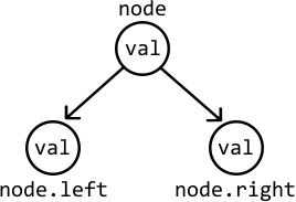
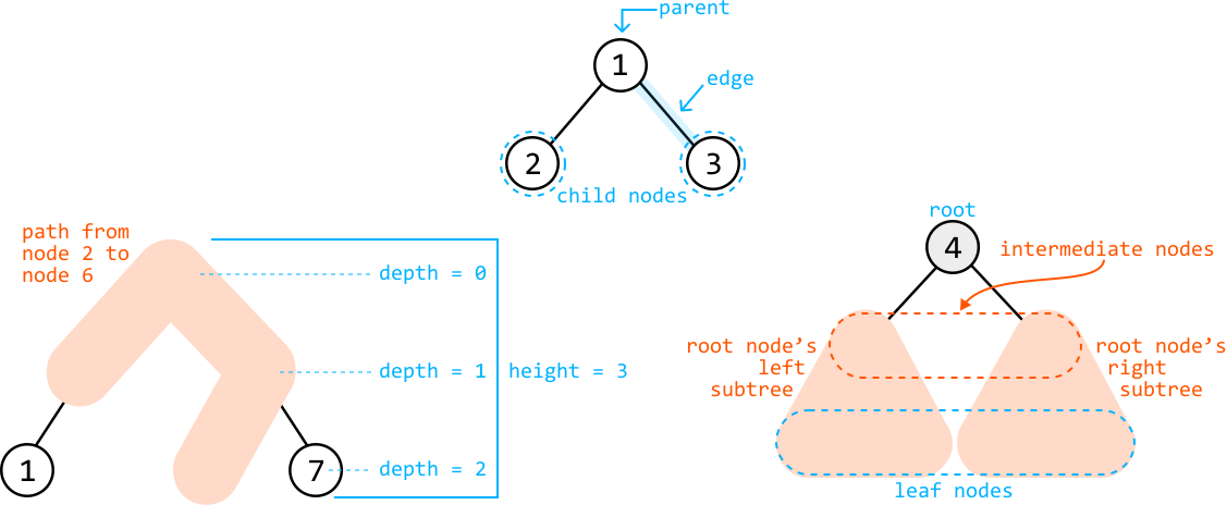
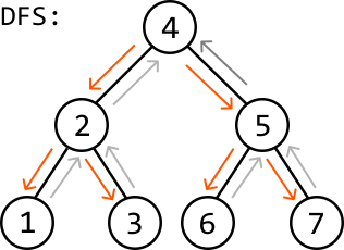
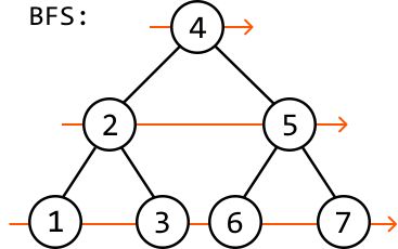
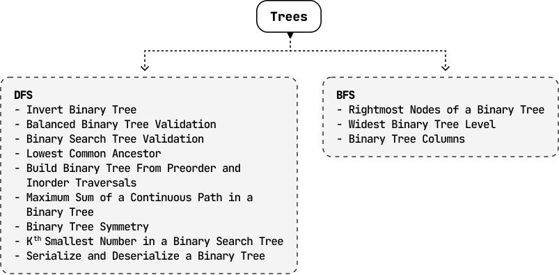
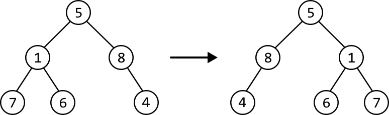
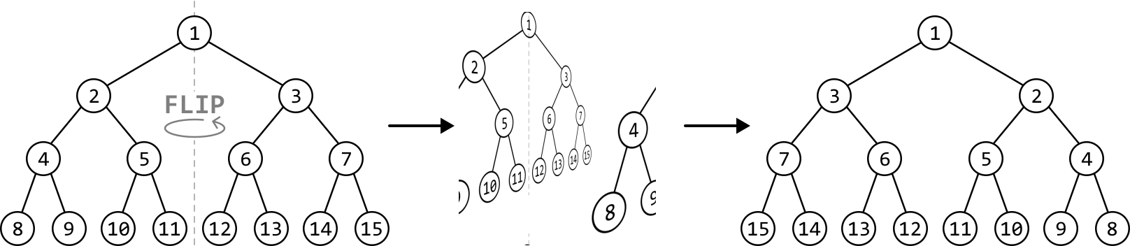
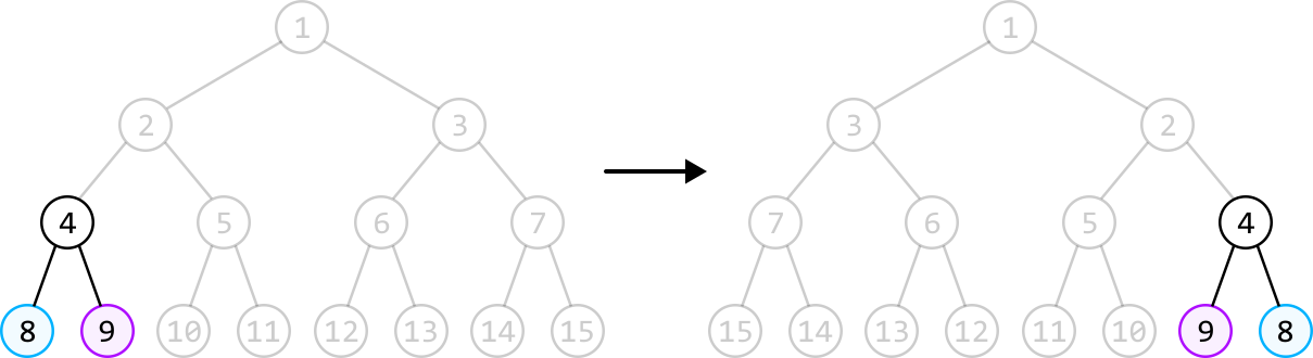
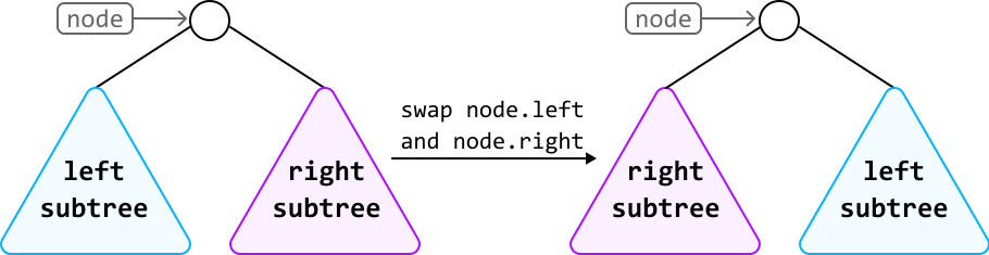
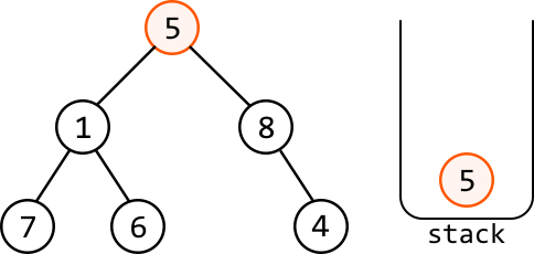
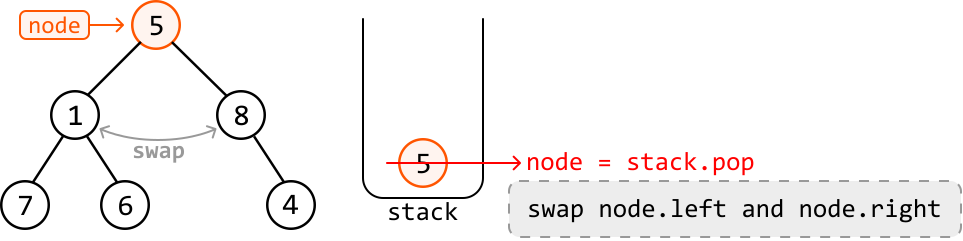
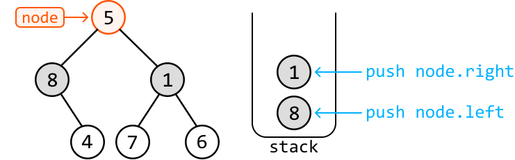
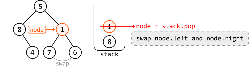
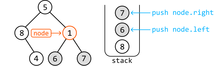
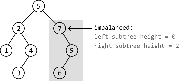
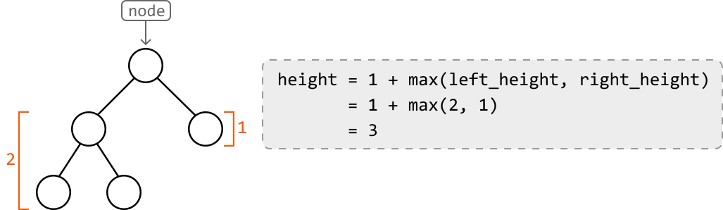
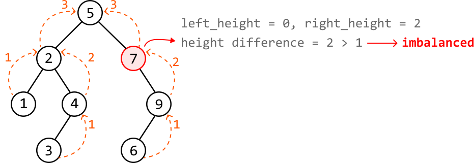
![Image represents a binary tree with nodes labeled numerically (1, 2, 3, 4, 5, 6, 8, 9, 11). Nodes 1, 3, and 6 are shaded gray and enclosed within a dashed oval, indicating a subset of the tree. Arrows indicate a traversal path from node 1 to node 3, and then to node 6. Node 11 is circled in red and a horizontal arrow points to it from the text 'missing,' highlighting its absence from the 'output' list. To the right, the 'output' is listed as `[1 3 6]`, while the 'expected output' is `[1 3 6 11]`, demonstrating that the algorithm represented by the tree traversal only produced a subset of the expected values, specifically omitting node 11. The tree structure shows a hierarchical relationship between the nodes, with node 1 as the root, and nodes 2 and 3 as its children. Node 2 has children 4 and 5, and node 4 has children 8 and 9. Node 3 has a child node 6, and node 5 has a child node 11.](images/img_1ffab9762d00.svg)
![Image represents a tree-like data structure, specifically a binary tree, on the left, and a queue data structure on the right. The binary tree is composed of circular nodes, each containing a single integer from 1 to 11. Node 1 is the root node, branching into nodes 2 and 3. Node 2 further branches into nodes 4 and 5, while node 3 connects to node 6. Node 4 branches into nodes 8 and 9, and node 5 connects to node 11. The connections between nodes represent parent-child relationships. On the right, a queue is depicted as `queue = [1]`, indicating that the queue currently contains only the integer 1, enclosed in square brackets. There is no visible connection or information flow between the tree and the queue; they are presented as separate structures.](images/img_88a3cb000b6a.svg)
![Image represents a visual explanation of Breadth-First Search (BFS) algorithm applied to a binary tree. The left side shows a binary tree with a root node labeled '1' (highlighted in peach), a left child node '2', and a right child node '3'. The nodes '2' and '3' have dashed lines indicating they might have further children, but these are not shown. A label 'Level 1:' precedes the root node. An arrow points from a rectangular box labeled 'node' to the root node '1', suggesting data flow into the algorithm. The right side demonstrates the algorithm's process. A queue, initially containing only node '1' (in a solid circle), is shown. A red arrow and the text 'node = queue.pop' indicate that node '1' is dequeued. Two blue arrows, labeled 'push node.left' and 'push node.right', show the left and right children ('2' and '3', respectively, in dashed circles) being enqueued into the queue, expanding the queue to '[2, 3]'. This illustrates the step-by-step process of BFS: visiting nodes level by level, adding children to the queue as they are encountered.](images/img_7d42e5959fe9.svg)
![Image represents a visual explanation of a breadth-first search (BFS) algorithm using a tree structure and a queue. A tree is shown with a root node labeled '1', connected to two child nodes labeled '2' and '3' at level 2. These child nodes are highlighted with a light peach-colored background, and the label 'Level 2:' is placed to their left. Dashed lines extend from nodes '2' and '3', suggesting further child nodes at subsequent levels, not explicitly shown. To the right, a queue is depicted as `queue = [2 3]`, indicating that nodes '2' and '3' are currently in the queue for processing. A light gray, dashed-line box below states 'size of queue = size of level 2', illustrating the relationship between the number of nodes in the queue and the number of nodes at the current level being processed in the BFS traversal.](images/img_86dbd736d219.svg)
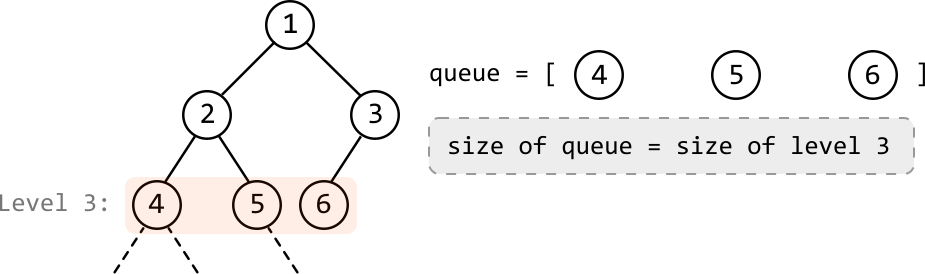
![Image represents a tree-like structure illustrating a coding pattern, possibly related to tree traversal or data collection. The tree has four levels, labeled 'Level 1,' 'Level 2,' 'Level 3,' and 'Level 4.' Each level contains nodes represented by circles, with numbers inside. Nodes 1, 3, 6, and 11 are highlighted with an orange border. Downward-pointing arrows indicate a traversal path, starting from node 1, then proceeding to nodes 3, 6, and finally 11. The nodes are connected by lines representing parent-child relationships. To the right, a list `res = [1 3 6 11]` shows the values collected during this traversal, suggesting that the algorithm collects values from the orange-highlighted nodes. The unhighlighted nodes (2, 4, 5, 8, 9) are part of the tree structure but are not included in the final result shown in the `res` list.](images/img_6b04820175c5.svg)
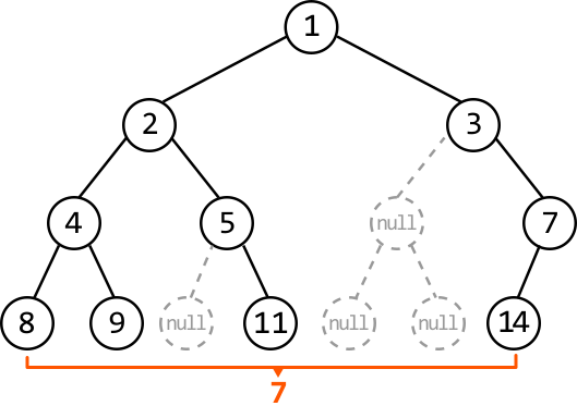
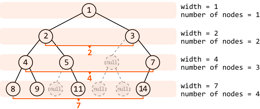
![Image represents a binary tree structure visualized across multiple horizontal layers, each representing a level of the tree. The nodes of the tree are circles containing numbers (1, 2, 3, 4, 5, 7, 8, 9, 11, 14), with orange numbers next to them indicating a sequential node numbering. Solid lines connect parent nodes to their children, illustrating the hierarchical relationships. Dashed lines and circles labeled '[null]' represent missing nodes or branches. To the right of the tree, calculations are shown for 'width' at each level. The formula used is `width = (largest node index - smallest node index) + 1`, with the result displayed below. For example, at the lowest level, the calculation is `width = (13 - 7) + 1 = 7`, reflecting the number of nodes (including nulls) present at that level. The top level has a width of 1, the second level has a width of 2, the third level has a width of 4, and the bottom level has a width of 7.](images/img_1dd497cb1361.svg)
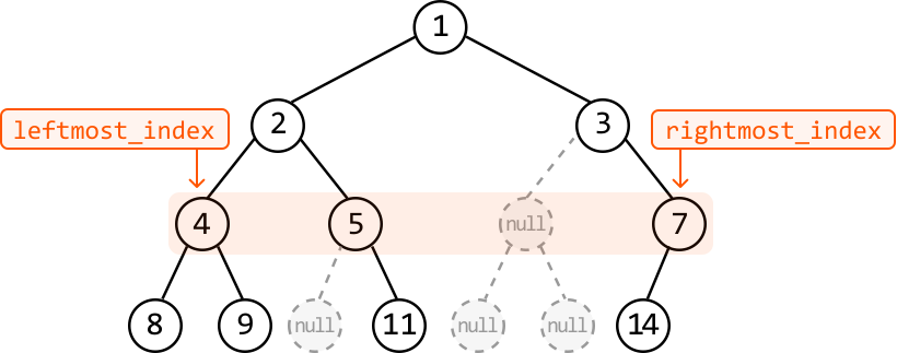
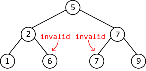
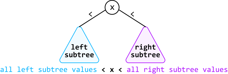
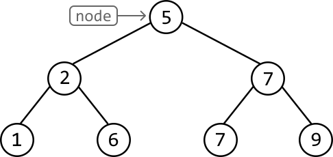
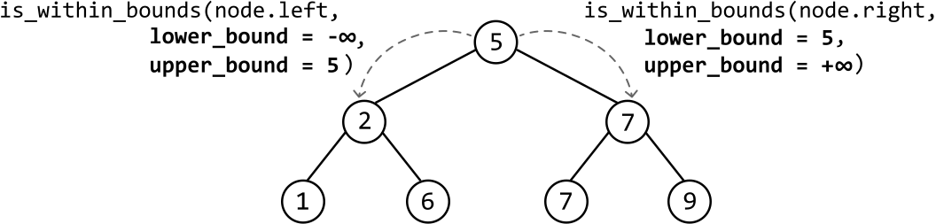
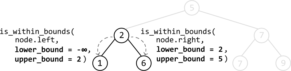
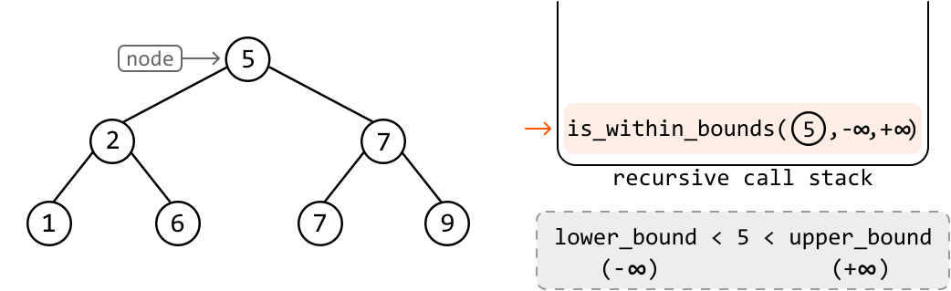
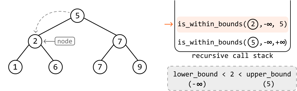
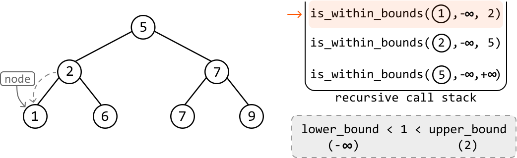
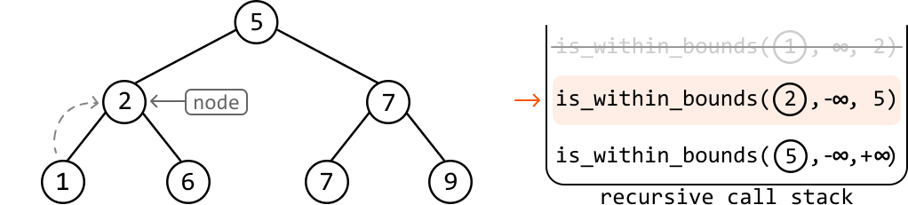
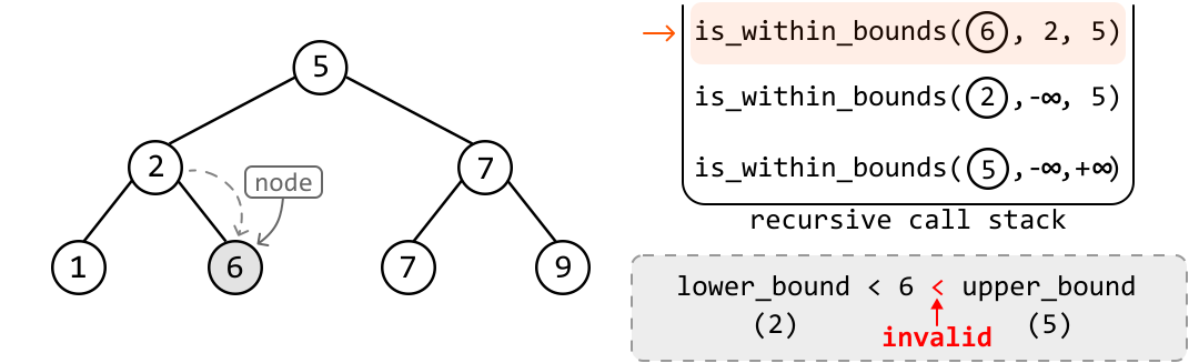
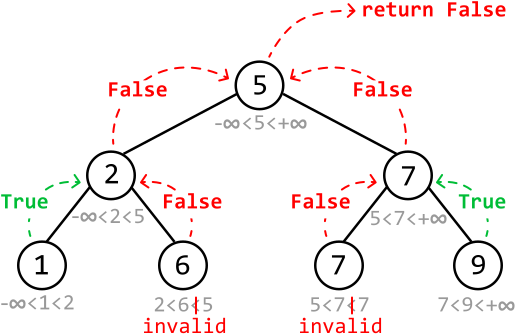
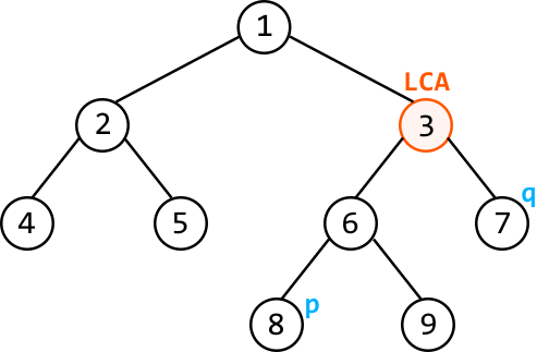
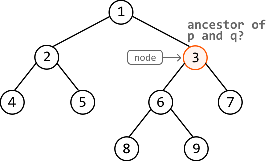
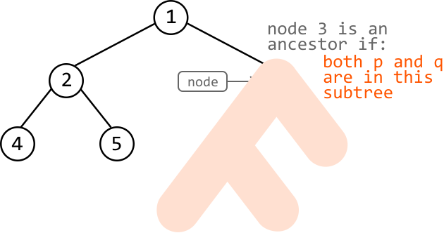
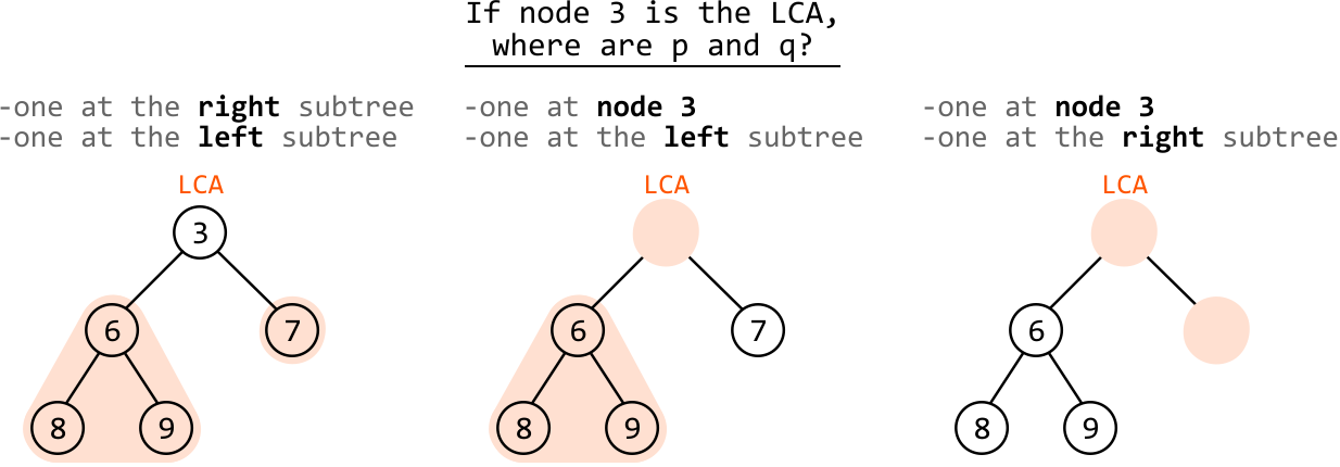
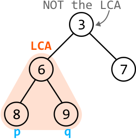
![Image represents three different binary trees, each visually depicted with nodes containing numerical values connected by branches, alongside an array labeled 'inorder = [2 9 5 4 3 7]'. The array represents an inorder traversal of all three trees. The first tree shows a root node '5' with a left subtree containing nodes '9' (parent) and '2' (child) and a right subtree with nodes '3' (parent), '4' (child), and '7' (child). The second tree has a root node '2', with a right subtree containing nodes '4' (parent), '5' (child), and '3' (child), where '3' has a right child '7' and '5' has a left child '9'. The third tree shows a root node '4', with a left subtree containing nodes '5' (parent), '2' (child), and '9' (child) and a right subtree with nodes '7' (parent) and '3' (child). All three trees contain the same set of nodes (2, 3, 4, 5, 7, 9), but their structures differ, demonstrating that different tree structures can yield the same inorder traversal.](images/img_eec8a67138f3.svg)
![Image represents a binary tree alongside its preorder and inorder traversal sequences. The right side shows a binary tree with root node '5'. Node '5' connects to a left child node '9' and a right child node '3'. Node '9' has a left child node '2', and node '3' has a left child node '4' and a right child node '7'. The left side displays two arrays: 'preorder' which lists the nodes in the order they are visited during a preorder traversal ([5, 9, 2, 3, 4, 7]), and 'inorder' which lists the nodes in the order they are visited during an inorder traversal ([2, 9, 5, 4, 3, 7]). The preorder traversal starts at the root and recursively visits the left subtree before the right subtree, while the inorder traversal recursively visits the left subtree, then the root, and finally the right subtree. The image demonstrates the relationship between a binary tree's structure and its preorder and inorder traversal sequences.](images/img_d2bdcb20ec1f.svg)
![Image represents a visual depiction of a preorder traversal in a tree structure. A rectangular box labeled 'root' in orange is positioned above an orange arrow pointing downwards towards a preorder array representation. The array, labeled 'preorder = [ 5 9 2 3 4 7 ]', shows a sequence of numbers. The number 5, the first element in the array, is highlighted by being enclosed in an orange circle below the array, indicating it's the root node of the tree. The arrow visually connects the 'root' label to the first element (5) of the preorder array, signifying that the value 5 is the root node of the tree whose preorder traversal is represented by the array. The remaining numbers in the array (9, 2, 3, 4, 7) represent the other nodes in the tree, ordered according to the preorder traversal algorithm (root, left subtree, right subtree).](images/img_2d7f6b4b7357.svg)
![Image represents a binary search tree with the root node labeled '5', highlighted in peach. The node '5' has a left subtree, shaded light blue, containing nodes '9' and '2', with '9' as the parent node and '2' as its child. A light orange arrow points from the inorder traversal array element '5' to the root node '5' in the tree. Similarly, the node '5' has a right subtree, shaded light purple, consisting of nodes '3', '4', and '7', where '3' is the parent node, and '4' and '7' are its left and right children respectively. A violet arrow points from the inorder traversal array element '3' to the node '3' in the tree. Above the tree, an inorder traversal array `[2, 9, 5, 4, 3, 7]` is shown, with the elements '2' and '9' representing the inorder traversal of the left subtree, '5' representing the root, and '4', '3', and '7' representing the inorder traversal of the right subtree. The text 'node 5's left subtree' and 'node 5's right subtree' clearly labels the respective subtrees. The arrows visually connect the inorder traversal array elements to their corresponding nodes in the tree, illustrating the relationship between the inorder traversal and the tree structure.](images/img_d4a2573d1252.svg)
![The image represents two possible binary tree structures derived from a preorder traversal sequence. At the top, a preorder traversal array is shown as `preorder = [5 9 2 3 4 7]`. A downward-pointing orange arrow highlights the number `9` within this array. Below the array, two small binary trees are presented. Both trees have a root node labeled `5` (in a black circle). The left tree shows a dashed line connecting the root node `5` to a child node `9` (in an orange circle), while the right tree shows the same root node `5` connected via a dashed line to a child node `9` (also in an orange circle). The word 'OR' is placed between the two trees, indicating that both structures are valid interpretations of the preorder traversal sequence given the ambiguity inherent in preorder traversals without additional information. The difference lies in which node is considered the child of the root node `5`.](images/img_f3315ae00248.svg)
![Image represents a diagram illustrating the construction of a binary tree from an inorder traversal array. The top line shows the inorder traversal array `inorder = [2 9 5 4 3 7]` split into two subarrays: `[2 9 5]` (highlighted in light blue) and `[4 3 7]` (highlighted in light purple). A light blue curved arrow connects the first subarray to the text 'left subarray not empty → left subtree exists,' indicating that the non-empty left subarray implies the existence of a left subtree in the corresponding binary tree. Similarly, a light purple curved arrow connects the second subarray to the text 'right subarray not empty → right subtree exists,' showing that the non-empty right subarray implies the existence of a right subtree. The diagram visually demonstrates how the presence of non-empty subarrays in an inorder traversal directly relates to the existence of left and right subtrees during binary tree construction.](images/img_dc95a81ec33a.svg)
![Image represents a visual explanation of constructing a binary tree from its preorder and inorder traversal sequences. The top section shows a labeled box 'preorder_index' pointing down to a preorder traversal sequence represented as `preorder = [5 9 2 3 4 7]`. Below this, another labeled box 'inorder_index' points to an inorder traversal sequence `inorder = [2 9 5 4 3 7]`, with the numbers 2 and 9 highlighted in light blue, and 4, 3, and 7 highlighted in light purple. To the right, a binary tree is depicted with the root node labeled '5'. The left subtree, represented by `[2,9]` in cyan, and the right subtree, represented by `[4,3,7]` in violet, branch from the root node. The diagram illustrates how the preorder and inorder sequences, along with their indices, are used to reconstruct the structure of the binary tree.](images/img_56a9d72b9e5a.svg)
![Image represents a diagram illustrating a recursive algorithm for constructing a binary tree from its preorder and inorder traversal sequences. At the top, a box labeled 'preorder_index' points down to a preorder traversal sequence represented as `preorder = [5 9 2 3 4 7]`. Below this, boxes labeled 'left' and 'right' branch from the preorder sequence. The 'left' box points to a portion of the inorder traversal sequence, `inorder = [2 9]`, highlighted in light blue, representing the left subtree. The 'right' box points to `inorder = [4 3 7]`, highlighted in lavender, representing the right subtree. Gray curved arrows connect the highlighted inorder subsequences to further subdivisions of the inorder sequence, indicated by `inorder = [2 9 5 4 3 7]` and `inorder = [2 9 5 4 3 7]`, respectively, with orange dashed lines showing the recursive partitioning of the inorder sequence to identify left and right subtrees. The numbers within the inorder sequences are used to locate the root of each subtree based on its position in the preorder sequence, recursively building the binary tree. The labels 'left' and 'right' consistently indicate the partitioning of the inorder sequence to define the left and right subtrees at each recursive step.](images/img_7fbadd6ef86c.svg)
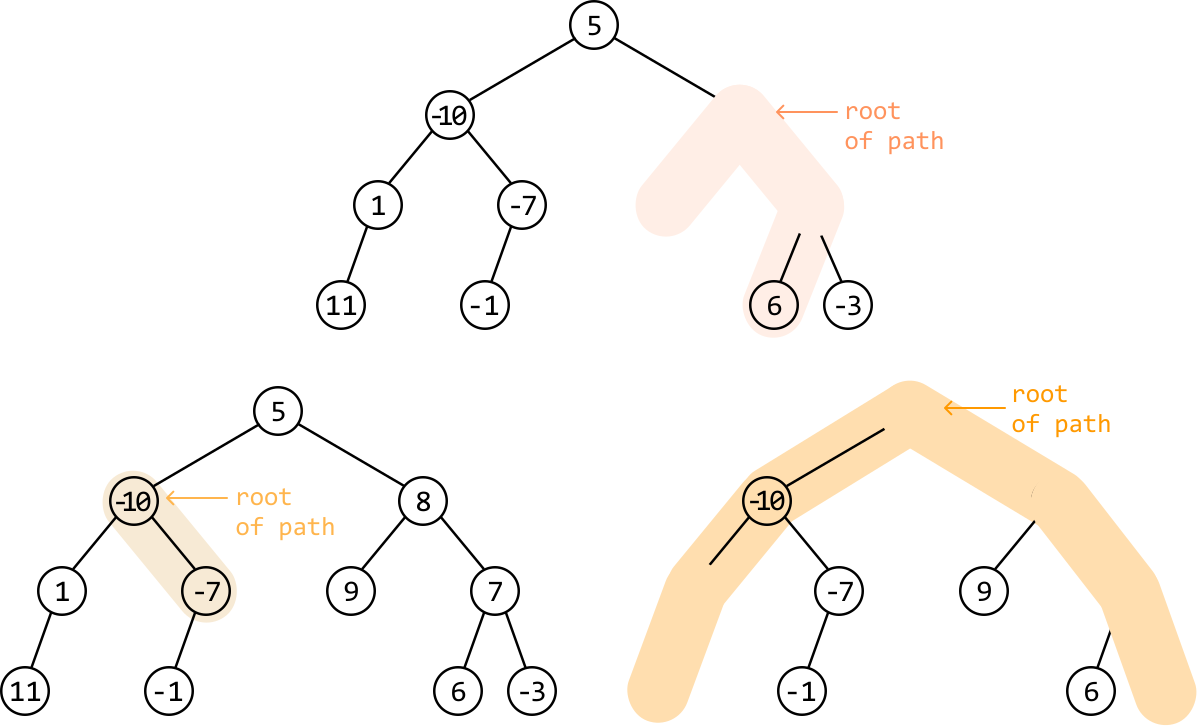
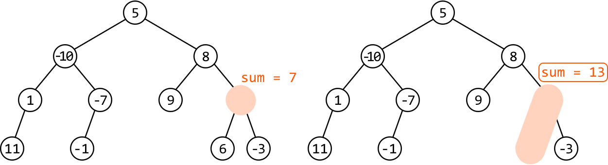
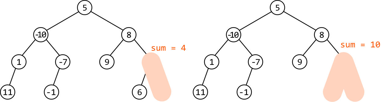
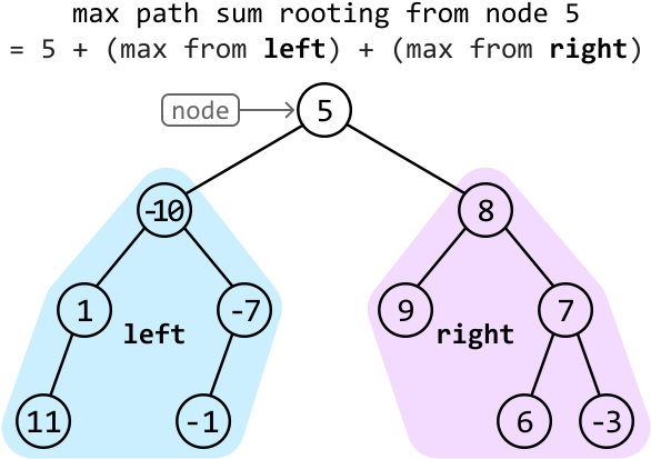
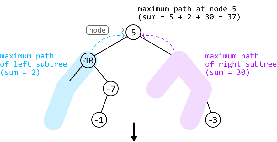
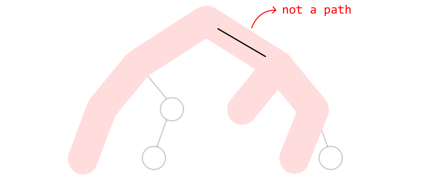
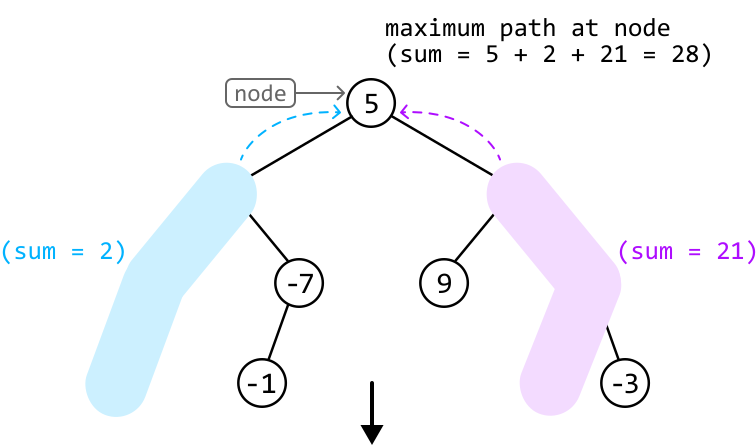
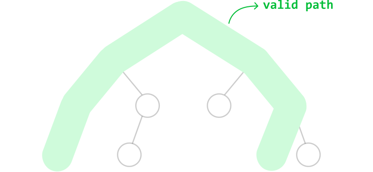
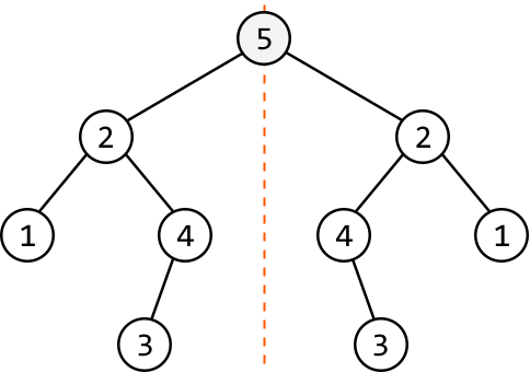
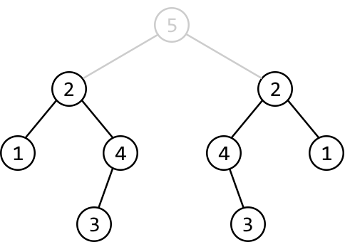
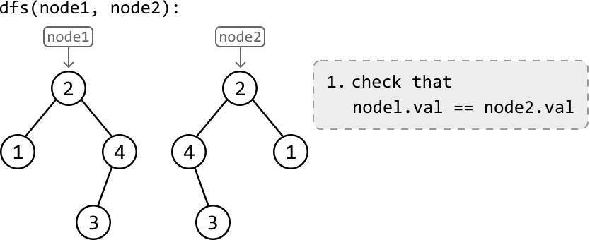
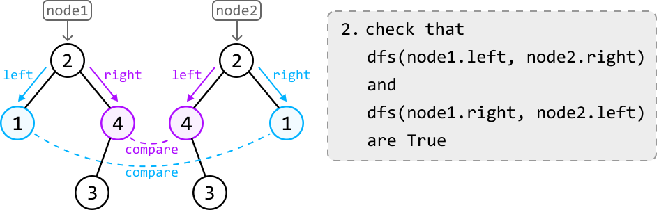
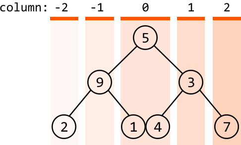
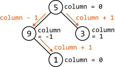
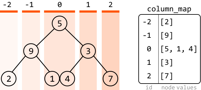
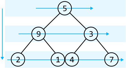
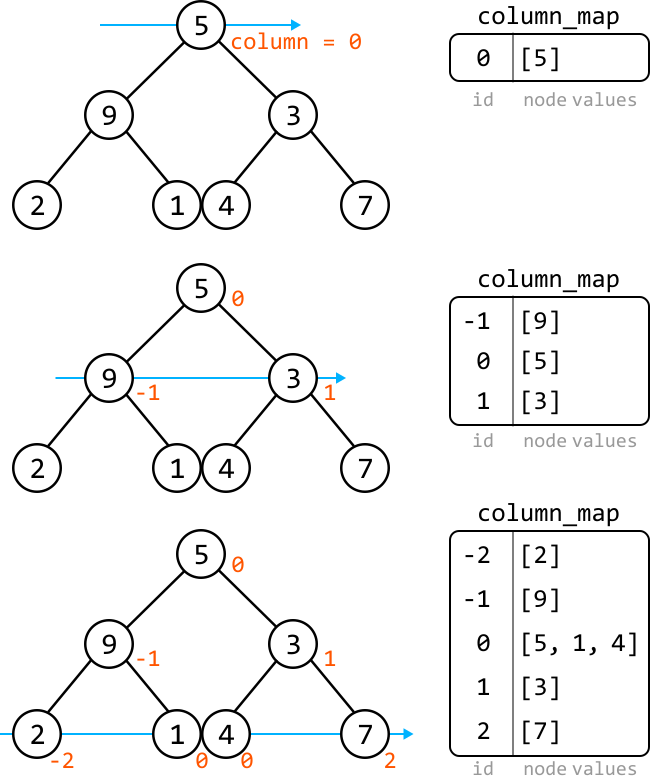
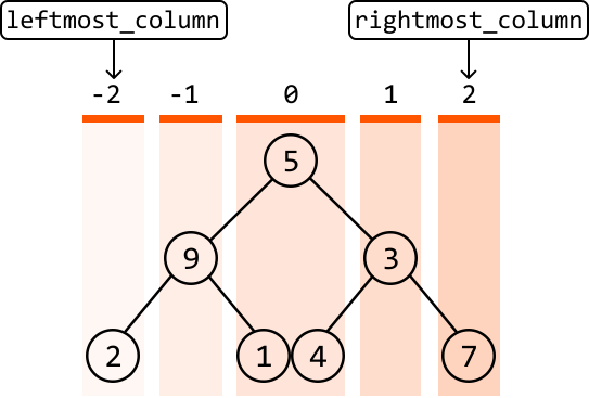
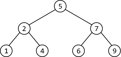
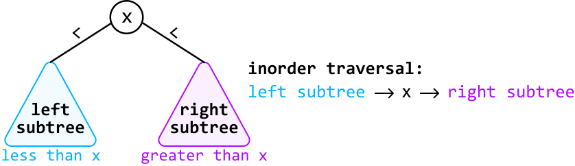
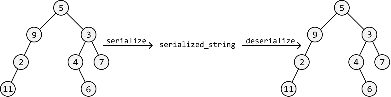
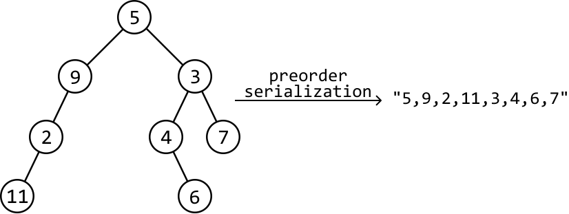
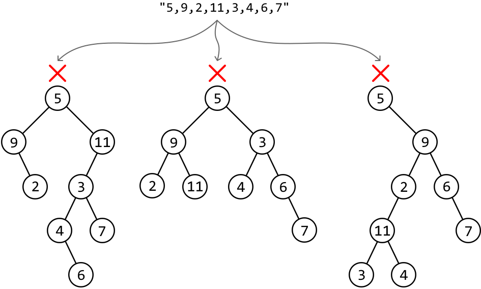
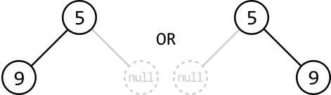
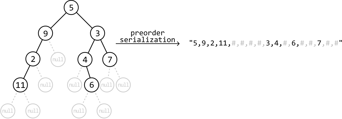
![Image represents a data transformation process illustrating the 'split' operation. At the top, a string '5,9,2,11,#,#,#,#,3,4,#,6,#,#,7,#,#' is shown. A downward-pointing arrow labeled 'split' connects this string to a list-like structure below. This list contains the same elements as the string, but arranged in a vertical array within square brackets `[]`. Each element from the original string is now on a separate line within the list. The '#' characters, representing null or placeholder values, maintain their positions relative to the numbers. The process visually demonstrates how a string of comma-separated values is split into individual elements, effectively transforming the string into a list or array data structure.](images/img_d16a959b98eb.svg)

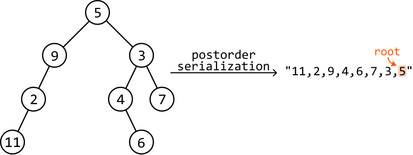
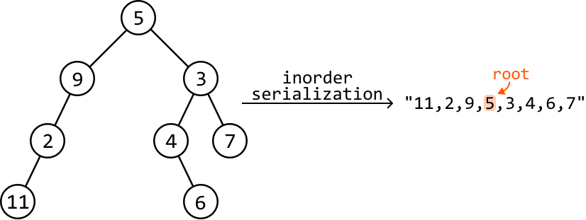
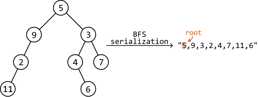

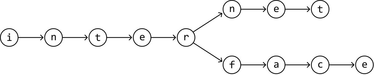
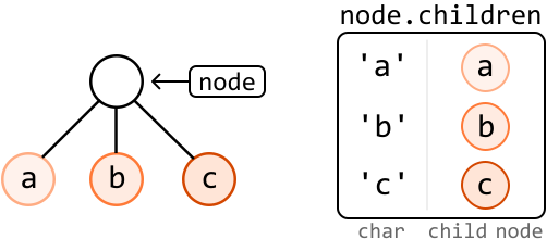
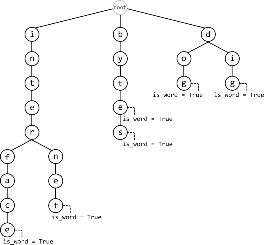
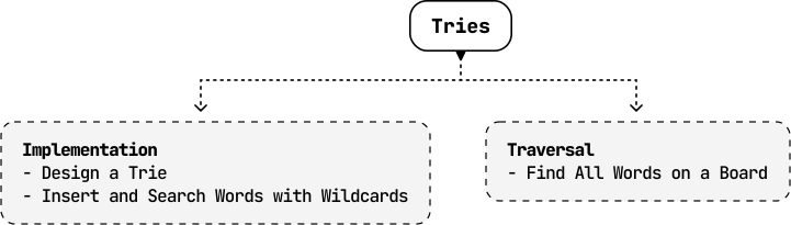
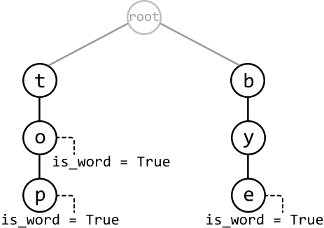
![Image represents a Trie data structure illustrating the insertion of the word 'byte'. The diagram shows a root node labeled 'root' (light gray) connected to two child nodes: 't' (black) and 'b' (orange). The 't' node branches down to 'o' and then 'p', each labeled with 'is_word = True', indicating these letter combinations are valid words. The 'b' node connects to 'y' and then 'e', also labeled 'is_word = True'. A dashed box to the right explains the insertion process: ' 'b' is a child of the current node' and the code snippet `node = node.children['b']` shows how the current node is updated to point to the 'b' node during insertion. A rectangular box labeled 'node' points to the root node initially, indicating the starting point of the insertion process. The lines connecting the nodes represent parent-child relationships within the Trie.](images/img_38100eebe995.svg)
![Image represents a tree-like data structure illustrating a coding pattern. The topmost node, labeled 'root' in light gray, branches into two nodes: 't' and 'b'. The 't' node connects downwards to 'o', which further connects to 'p'. Dashed lines connect 'o' and 'p' to the text 'is_word = True', indicating a property associated with these nodes. Similarly, the 'b' node connects to a node 'y' highlighted in orange, which then connects to 'e'. 'e' also has a dashed line connecting it to 'is_word = True'. A rectangular box to the right shows the code snippet `'y' is a child of the current node => node = node.children['y']`, explaining how to access the child node 'y' from a parent node (represented by the variable 'node'). A smaller rectangular box labeled 'node' points to the 'b' node, illustrating the current node in the example. The overall structure depicts a Trie or prefix tree, commonly used in data structures and algorithms, particularly for efficient string searching.](images/img_d20e9cf3bf18.svg)
![Image represents a Trie data structure visualization alongside code snippets illustrating its modification. The Trie is depicted as a tree with a light-grey root node labeled 'root'. Two branches extend from the root, leading to nodes labeled 't' and 'b' respectively. The 't' node connects to an 'o' node, which in turn connects to a 'p' node. Both 'o' and 'p' nodes have dashed lines indicating a boolean attribute 'is_word = True'. The 'b' node connects to a 'y' node, which further connects to an 'e' node. The 'e' node also has a dashed line indicating 'is_word = True'. A dashed line connects the 'y' node to a new, orange-colored 't' node, representing a node being added. A rectangular box to the right displays code comments explaining that 't' is not a child of the current node ('y'), followed by two lines of code: `node.children['t'] = TrieNode()` which creates a new TrieNode for 't', and `node = node.children['t']` which updates the current node pointer to the newly created 't' node. A separate rectangular box labeled 'node' points to the 'y' node, indicating the current node before the addition of the 't' node.](images/img_f67edd225495.svg)
![Image represents a Trie data structure illustrating the insertion of a new node. The Trie is visualized as a tree with a light gray root node labeled 'root'. From the root, two branches extend to nodes labeled 't' and 'b'. The 't' node connects to an 'o' node, which in turn connects to a 'p' node. Both 'o' and 'p' nodes have a dashed line and label 'is_word = True', indicating they represent complete words. The 'b' node connects to a 'y' node, which further branches to 'e' and 't' nodes. The 'e' node has 'is_word = True'. A dashed line connects the 't' node to a new, orange-colored 'e' node, labeled 'node', signifying the addition of this node. A separate box explains the process: ''e' is not a child of the current node' followed by two lines of code: '→ node.children['e'] = TrieNode()' and '→ <font color='orange'>node</font> = node.children['e']', showing how a new TrieNode is created and assigned to the 'e' child of the current node. The arrows indicate the flow of information and the creation of a new node within the Trie.](images/img_df2062c03e2e.svg)
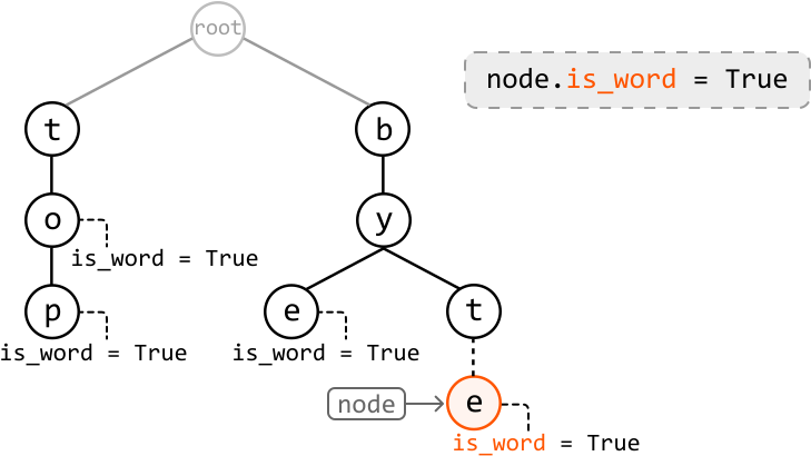
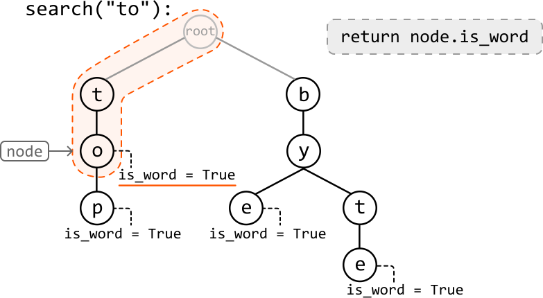
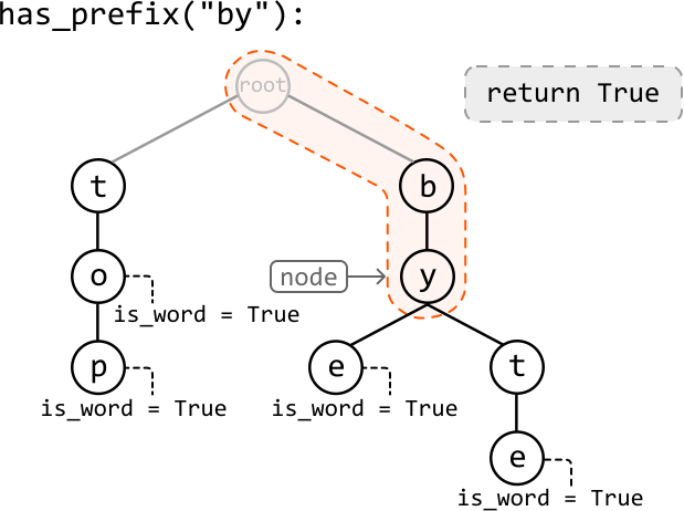
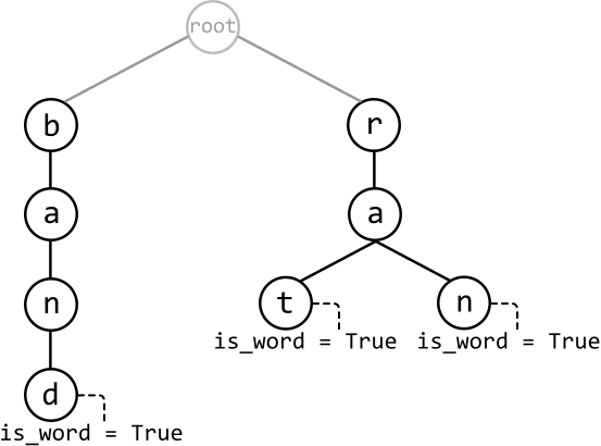
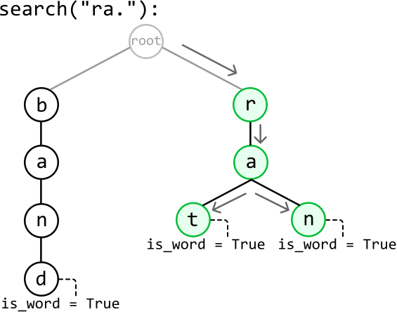
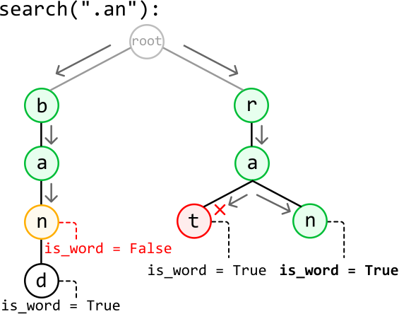
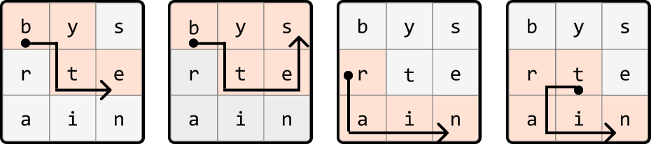
![Image represents a Trie data structure visualizing the storage of the words ['byte', 'rat', 'rain', 'bytes', 'trait', 'train']. A root node labeled 'root' branches into three main paths. The leftmost path, using dark-colored nodes, spells out 'bytes,' with each node representing a letter (b, y, t, e, s). Dashed lines connect the end nodes to labels indicating the complete words formed ('byte' and 'bytes'). The central path, also using dark-colored nodes, initially spells 'rat' (r, a, t), with a dashed line and label indicating the complete word. This path further extends to 'rain' (r, a, i, n) using a lighter-colored node for 'i' and 'n', again with a dashed line and label. The rightmost path, using dark-colored nodes, spells 'train' (t, r, a, i, n), with the final 'n' node having a dashed line and label indicating the complete word. The lighter-colored nodes in the 'rain' and 'train' paths indicate shared prefixes with other words in the Trie. The top line shows the Python list containing all the words stored in the Trie.](images/img_7cd0b37fd8cd.svg)
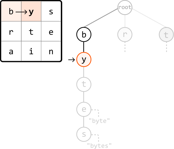
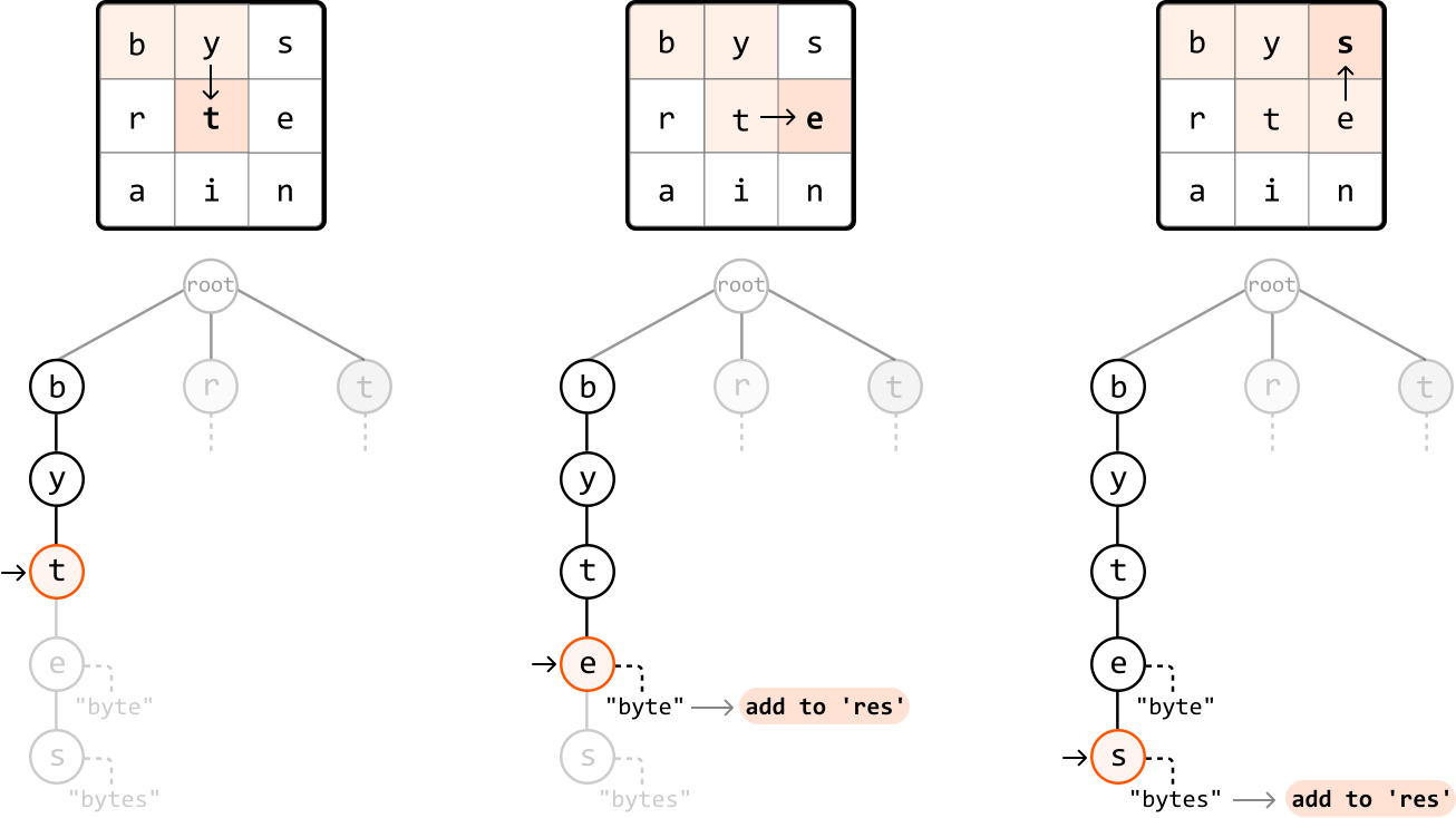
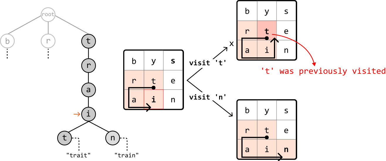
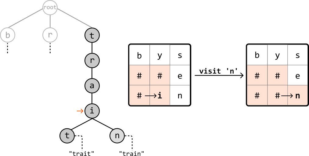


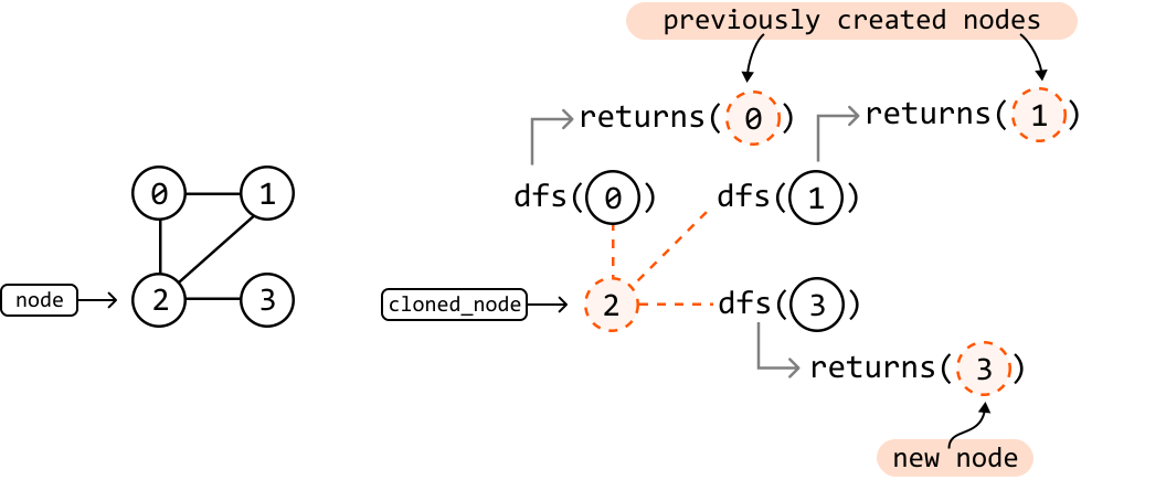
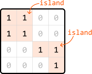
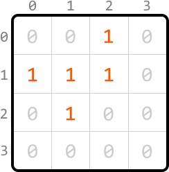
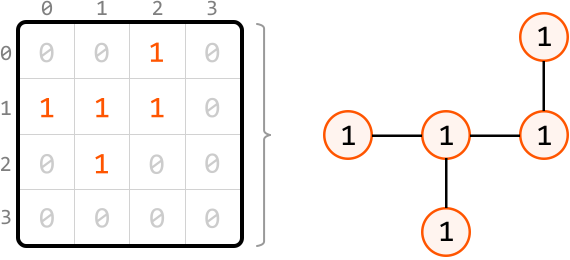
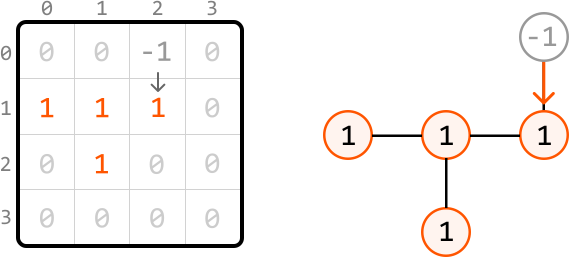
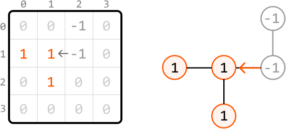
![Image represents a comparison between a matrix representation and a graph representation of data. On the left, a 4x4 matrix is shown with numerical values. Rows and columns are labeled 0-3. Most cells contain '0' (in light gray), but some contain '1' (in orange) and '-1' (in dark gray). Specifically, a '1' is located at matrix[1][0] and matrix[2][1]. A '-1' is present at matrix[0][2], matrix[1][1], and matrix[1][2]. An arrow points to the '1' at matrix[1][0], indicating a potential focus or starting point. On the right, a directed acyclic graph is displayed. Nodes represent numerical values; orange circles represent '1', and gray circles represent '-1'. Edges connect the nodes, showing relationships. An orange arrow points from a '1' node to a '-1' node, indicating a directional flow. The graph visually represents the connections and relationships between the non-zero elements in the matrix, with the orange '1' nodes corresponding to the '1's in the matrix and the gray '-1' nodes corresponding to the '-1's in the matrix. The structure suggests a possible flow or dependency between the data points.](images/img_77b0e5988cd3.svg)
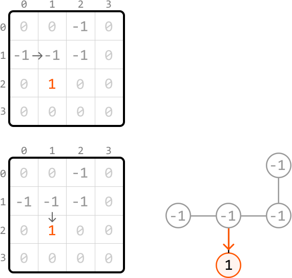
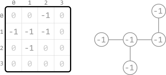
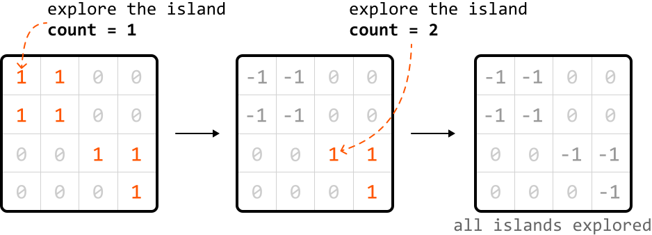
![Image represents a visual explanation of how to move in four directions (Up, Down, Left, Right) on a 2D grid using array indexing. The left side shows four equations, each representing a directional movement. Each equation takes a coordinate pair (r, c) representing the row and column of a cell and adds it to an element from a `dirs` array. `dirs[0]` corresponds to moving Up, resulting in (r - 1, c); `dirs[1]` corresponds to moving Down, resulting in (r + 1, c); `dirs[2]` corresponds to moving Left, resulting in (r, c - 1); and `dirs[3]` corresponds to moving Right, resulting in (r, c + 1). The right side displays a 3x3 grid visually illustrating these movements. The central cell is highlighted in light gray and labeled (r, c), representing the starting point. The surrounding cells are labeled with their respective coordinates, showing the result of applying the directional equations. The grid demonstrates the effect of adding the `dirs` array elements to the initial coordinate (r, c) to obtain the new coordinates after moving in a specific direction.](images/img_728d3af0d817.svg)

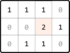
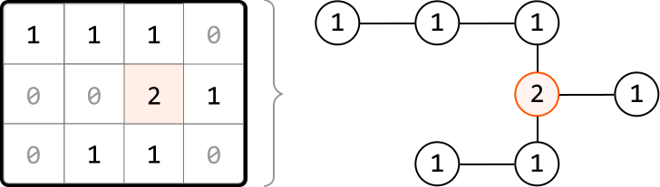
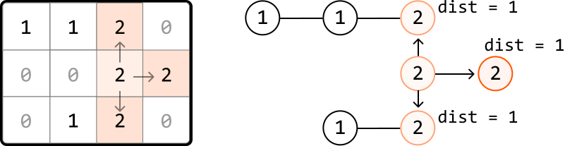
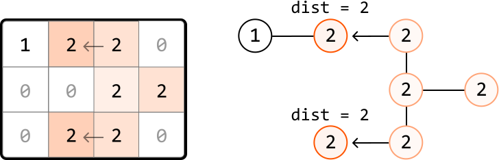
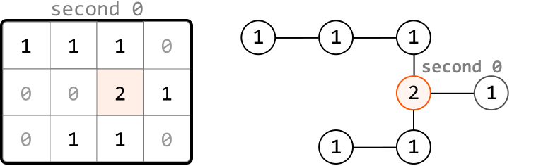
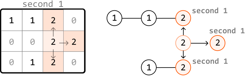
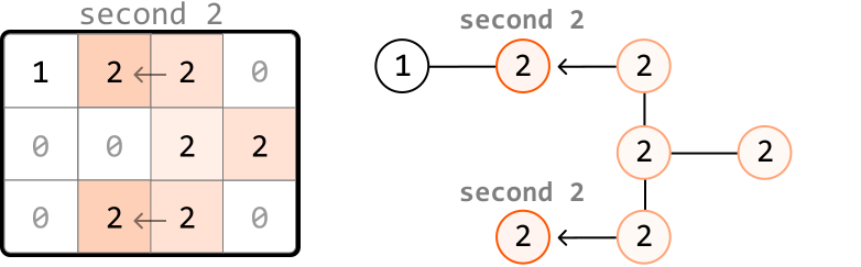
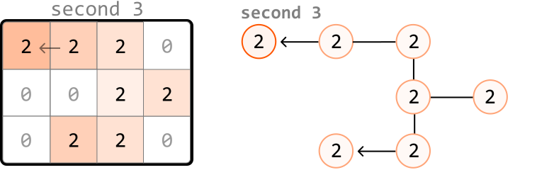
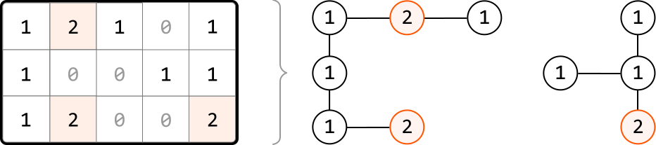
![Image represents a 3x5 matrix where each cell contains a numerical value. The rows are labeled 0, 1, and 2, and the columns are labeled 0, 1, 2, 3, and 4. The matrix cells contain the numbers 0, 1, and 2, with some cells highlighted in a light peach color. These highlighted cells represent elements that are part of a queue, which is defined to the right of the matrix as `queue = [(0, 1) (2, 1) (2, 4)]`. This queue notation indicates that the coordinates (row, column) of the highlighted cells are (0,1), (2,1), and (2,4). The numbers within the matrix cells themselves do not appear to directly relate to the queue's structure; rather, the queue identifies specific cell locations within the matrix.](images/img_d8d9b9515abb.svg)
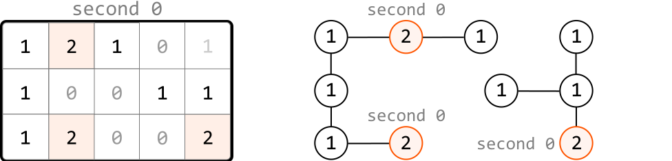
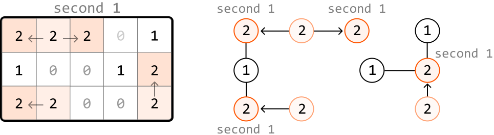
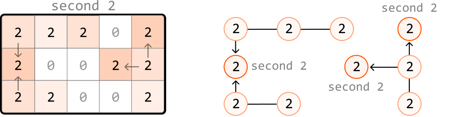
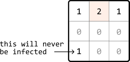
![Image represents a 3x3 matrix alongside a queue and a count. The matrix is indexed with row and column numbers from 0 to 2. The matrix cells contain integers; a '2' is highlighted in a peach/light-orange color at row 0, column 1. Other cells contain '1's and '0's. To the right of the matrix, a queue is defined as `queue = [(0, 1)]`, representing a coordinate pair (row, column) indicating the position of the highlighted '2'. Finally, a count `ones = 3` indicates the total number of '1's present within the matrix. The matrix, queue, and count likely represent an intermediate state in an algorithm, possibly related to searching or processing a 2D array.](images/img_5706d813d625.svg)
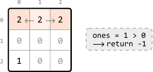
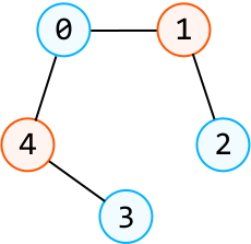
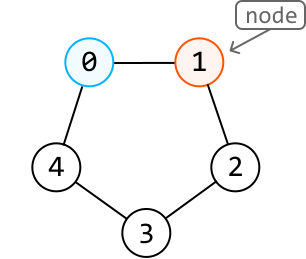
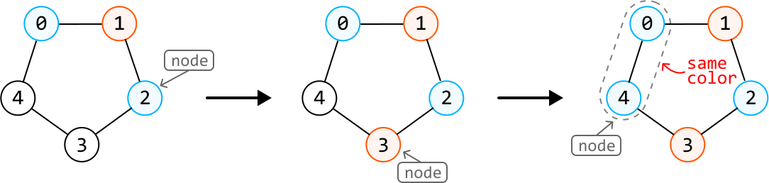
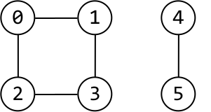
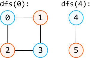
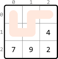
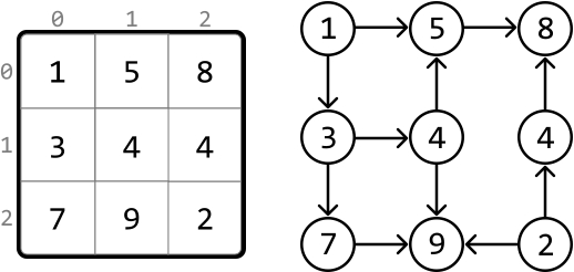
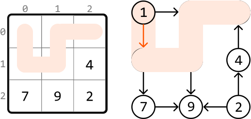
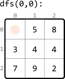
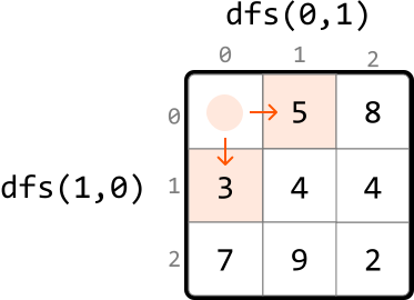
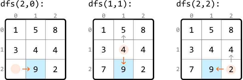

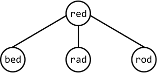
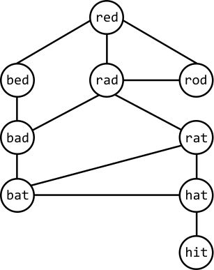
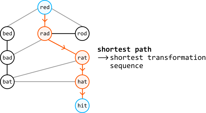
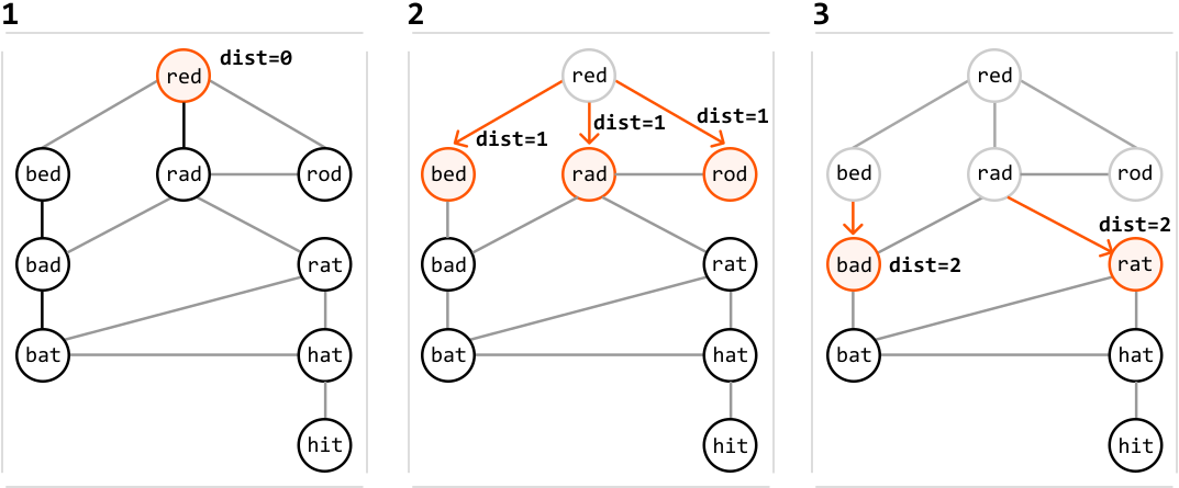
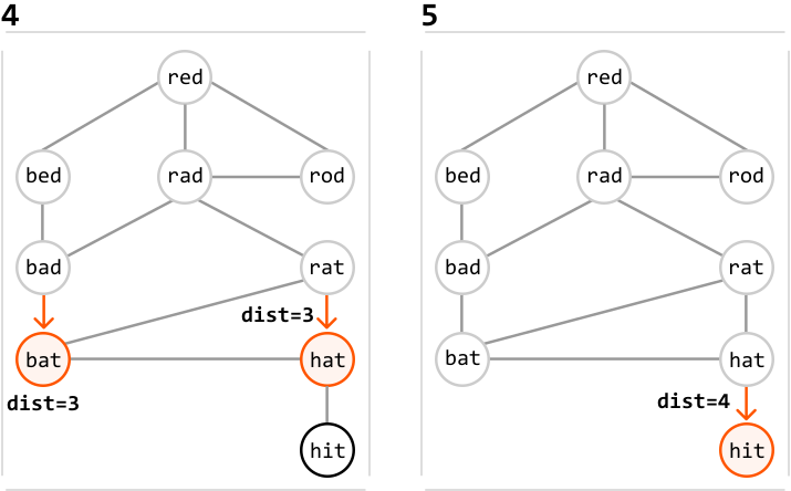
![Image represents a graph data structure depicted in a textual format. The text is labeled 'graph:' and presents a series of key-value pairs. Each key is a string enclosed in double quotes (e.g., 'red'), representing a node in the graph. The value associated with each key is a list of strings, also enclosed in square brackets, representing the nodes directly connected to the key node (its neighbors). For instance, 'red': [ 'bed', 'rad', 'rod'] indicates that the node 'red' is connected to nodes 'bed', 'rad', and 'rod'. Similarly, 'bed' connects to 'red' and 'bad', 'hat' connects to 'rat', 'bat', and 'hit', and 'hit' connects only to 'hat'. The ellipsis (...) suggests that there might be more key-value pairs not shown in the image, implying a larger graph. The overall structure represents an adjacency list representation of a directed or undirected graph, depending on whether the connections are considered bidirectional.](images/img_76b5b97ba026.svg)
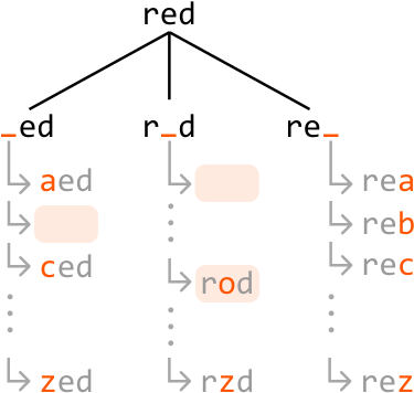
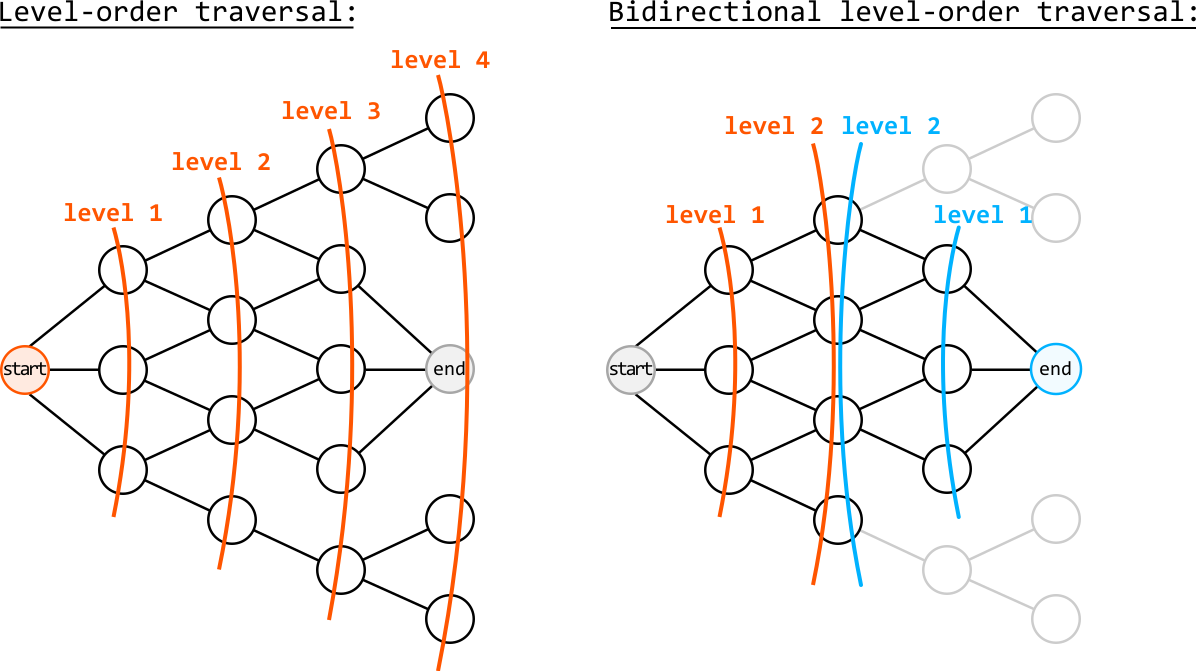
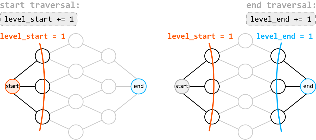
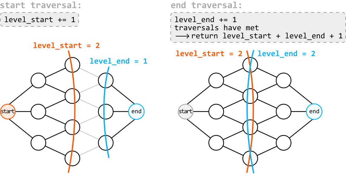
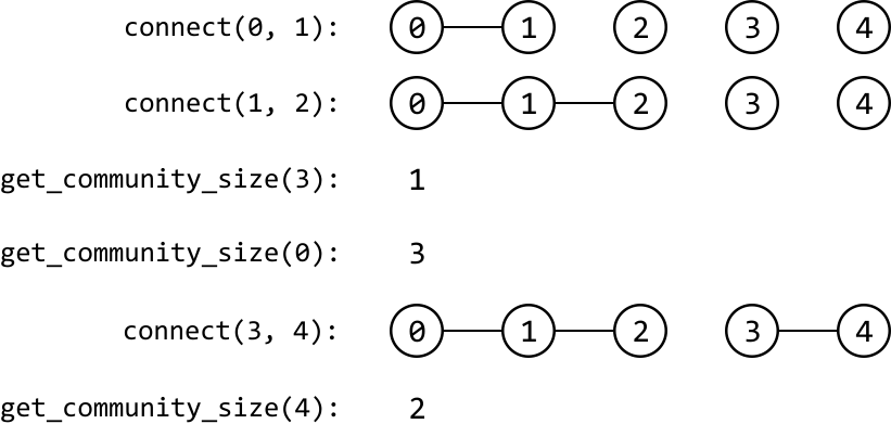
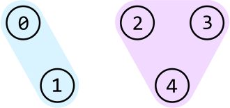
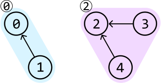
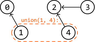
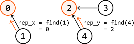
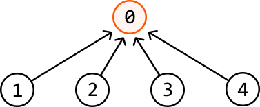
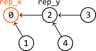
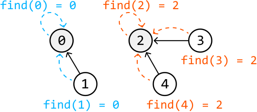
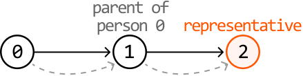
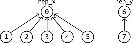
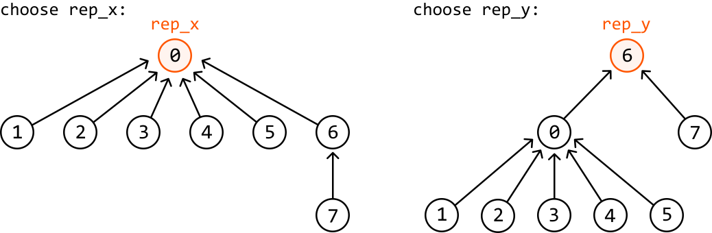
![Image represents a tree-like data structure illustrating a 'find' operation within a disjoint-set data structure, likely used for representing sets and their relationships. The central node, labeled '0' and highlighted in orange, is the representative element ('rep') of the entire set. Nodes 1 through 6 represent other elements within the set. Solid black arrows indicate the parent-child relationships within the structure; for example, node 2 is a child of node 1, and node 1 is a child of node 0. Dashed gray arrows represent the path a 'find(parent[i])' operation would take to locate the representative element for a given node 'i'. For instance, `find(parent[3])` would traverse from node 3 to node 2, then to node 1, and finally to node 0 (the representative). Each leaf node (3 and 6) has a label indicating a `find(i)` operation, suggesting a direct path to find the element itself. The overall structure shows how the `find` operation navigates the tree to identify the representative element of a given node's set.](images/img_349d5132b49e.svg)
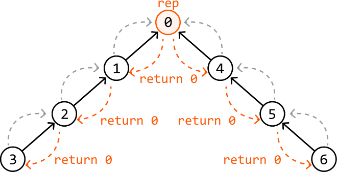
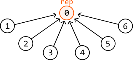
![Image represents a directed graph illustrating prerequisites, where `prerequisites = [[0, 1], [1, 0]]` defines the dependencies. The graph consists of two nodes, represented by circles labeled '0' and '1'. A directed edge, indicated by an arrow, connects node '0' to node '1', signifying that node '1' requires node '0' as a prerequisite. Conversely, another directed edge connects node '1' to node '0', indicating a reciprocal dependency; node '0' also requires node '1'. The `prerequisites` array is a matrix where each inner array represents a dependency; `[0, 1]` means 1 depends on 0, and `[1, 0]` means 0 depends on 1. This visual representation shows a cyclical dependency between the two nodes.](images/img_f58b7dc2431f.svg)
![Image represents two directed graphs illustrating different prerequisite relationships. Each graph contains three nodes labeled '0', '1', and '2', representing tasks or modules. Arrows indicate dependencies; an arrow from node A to node B signifies that B requires A as a prerequisite. The left graph shows node 0 pointing to node 1, node 1 pointing to node 2, and node 2 pointing back to node 1, representing a cyclical dependency. Above this graph, the text 'prerequisites = [[0,1] [1,2] [2,1]]' lists these dependencies as ordered pairs within a list of lists. The right graph shows node 0 pointing to node 1, node 1 pointing to node 2, and node 2 pointing to node 0, forming a different cyclical dependency. Above this graph, the text 'prerequisites = [[2,0] [0,1] [1,2]]' similarly lists the dependencies as ordered pairs in a list of lists, reflecting the connections in the graph. Both graphs visually represent different sets of prerequisites, highlighting how different dependency structures can be represented using directed graphs and their corresponding list representations.](images/img_ebbe1b2d8479.svg)
![Image represents a directed graph illustrating prerequisites. The graph consists of six nodes, numbered 0 through 5, represented as circles containing their respective numbers. Arrows indicate directed edges showing dependencies; a directed edge from node *x* to node *y* means *y* depends on *x*. The edges are labeled with small orange numbers, possibly representing weights or costs associated with the dependencies. Specifically, node 0 has outgoing edges to nodes 1 and 2; node 1 has an outgoing edge to node 4; node 3 has an outgoing edge to node 2; node 2 has an outgoing edge to node 4; and node 4 has an outgoing edge to node 5. Above the graph, a Python list named `prerequisites` is defined, containing nested lists. Each nested list represents a dependency pair; for example, `[0,1]` indicates that node 1 depends on node 0. The list explicitly defines all the dependencies shown in the graph.](images/img_5dbcc49f3d97.svg)
![Image represents a directed graph illustrating prerequisites. At the top, a Python list named `prerequisites` is defined, containing pairs of numbers representing dependencies: `[[0,1] [0,2] [3,2] [1,4] [2,4] [4,5] [5,2]]`. The graph visually depicts these dependencies. The graph consists of six nodes, numbered 0 through 5, represented as circles containing their respective numbers. Directed edges, represented by arrows, connect the nodes, indicating the flow of dependencies. For example, the edge from node 0 to node 1 (labeled with an orange '1' above the arrow) signifies that node 1 requires node 0 as a prerequisite. Similarly, node 2 requires node 0 (labeled '0'), node 2 requires node 3 (labeled '3'), node 4 requires node 1 (labeled '2'), node 4 requires node 2 (labeled '1'), node 5 requires node 4 (labeled '1'), and node 2 requires node 5 (a curved edge). The numbers on the arrows correspond to the order of dependencies as listed in the `prerequisites` list.](images/img_70f3d3815bd6.svg)

![Image represents a directed acyclic graph (DAG) illustrating a topological sort problem, along with its prerequisites and in-degrees. The upper part shows the DAG with six nodes (0, 1, 2, 3, 4, 5) represented as circles, connected by directed edges indicated by arrows. The numbers on the arrows represent edge weights (not explicitly defined but implied). Node 0 points to node 1 and node 2; node 3 points to node 2; node 1 points to node 4; and node 4 points to node 5. Below the DAG, a list named 'prerequisites' shows the dependencies as pairs of node indices: `[[0,1] [0,2] [3,2] [1,4] [2,4] [4,5]]`, indicating that node 1 requires node 0, node 2 requires node 0, node 2 requires node 3, node 4 requires node 1, node 4 requires node 2, and node 5 requires node 4. Finally, a list named 'in_degrees' shows the number of incoming edges for each node: `[0 1 2 0 2 1]`, indicating that node 0 has 0 incoming edges, node 1 has 1, node 2 has 2, and so on. Orange curved arrows connect the prerequisites pairs to their corresponding in-degree values in the `in_degrees` list, visually linking the dependencies to the count of incoming edges for each node. The numbers below the `in_degrees` list (0, 1, 2, 3, 4, 5) correspond to the node indices.](images/img_3e6578bf1179.svg)
![Image represents a directed acyclic graph (DAG) with five nodes (0, 1, 2, 3, 4) and edges connecting them, along with an accompanying illustration of a topological sort algorithm's execution. The nodes are numbered 0 through 4 and are depicted as circles containing their respective numbers. Edges are represented by arrows indicating direction; for example, node 0 points to node 1, and node 3 points to node 2. Small orange numbers next to each edge indicate a weight or some associated value. The algorithm uses an `in_degrees` array, shown as `[0 1 2 0 2 1]`, representing the number of incoming edges for each node (node 0 has 0 incoming edges, node 1 has 1, and so on). A `queue` array, initialized as `[0 3]`, stores nodes with zero incoming edges. A light green highlight visually emphasizes the current state of the `in_degrees` array, showing that nodes 0 and 3 are initially in the queue because they have no incoming edges. The graph's structure and the `in_degrees` and `queue` arrays together illustrate the data structures used in a topological sorting algorithm.](images/img_7e287b88a6a9.svg)
![Image represents a directed acyclic graph (DAG) illustrating a topological sort algorithm. The DAG consists of five nodes (circles) numbered 1 through 5, with directed edges (arrows) indicating dependencies. Node 0 is shown in gray and crossed out, indicating it's a source node that has been processed. A directed edge from node *i* to node *j* implies that node *j* depends on node *i*. The edges are labeled with small numbers representing weights or counts (e.g., 1→0, 2→1). To the right, an array named `in_degrees` is shown, representing the in-degree of each node (number of incoming edges). Initially, `in_degrees` is [0, 1, 2, 0, 2, 1], with node 0's in-degree crossed out because it's processed. Another array, `queue`, is shown as [0, 3], indicating nodes with an in-degree of 0 (ready to be processed). The orange numbers on the nodes and edges likely represent the order of processing during the topological sort. The graph visually demonstrates the flow of information and dependencies, with the arrays tracking the algorithm's progress.](images/img_0024134e3e1a.svg)

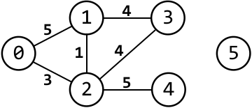
![Image represents a weighted, undirected graph with six nodes (labeled 0 through 5) and several edges connecting them. The edges are labeled with their corresponding weights. Node 0 connects to node 1 (weight 5) and node 2 (weight 3). Node 1 connects to node 2 (weight 1), node 3 (weight 4), and node 0 (weight 5). Node 2 connects to node 4 (weight 5) and node 3 (weight 4). Node 3 connects to node 1 (weight 4). Node 4 and node 5 are isolated nodes, not connected to any other nodes in the graph. To the right of the graph, a list named 'distances' is shown, initialized as `[0, ∞, ∞, ∞, ∞, ∞]`. The numbers below the list (0, 1, 2, 3, 4, 5) correspond to the indices of the nodes in the graph, indicating that the list represents the distances from a starting node (likely node 0, given the initial 0 in the list) to each of the other nodes in the graph. The symbol ∞ represents infinity, signifying that initially, the distances to nodes other than the starting node are considered unreachable.](images/img_7d58c8ebacd8.svg)
![Image represents a weighted graph illustrating a shortest path algorithm, possibly Dijkstra's algorithm. The graph consists of six nodes (0-5), with node 0 labeled 'curr' and colored orange, indicating a starting node. Nodes 1 and 2 are light blue, suggesting they've been visited. The remaining nodes (3, 4, 5) are unvisited. Edges connecting the nodes are labeled with their respective weights (1, 3, 4, 5). For instance, node 0 connects to node 1 with a weight of 5 and to node 2 with a weight of 3. Node 1 connects to node 2 with a weight of 1 and to node 3 with a weight of 4. Node 2 connects to node 4 with a weight of 5. Node 3 connects to node 1 with a weight of 4. To the right, a distances array `[∞ ∞ ∞ ∞ ∞ ∞]` is shown, representing the initial distances from the source node (0) to all other nodes, where ∞ denotes infinity. The array is partially updated, showing distances 5 and 3, calculated from the source node to nodes 1 and 2 respectively, indicated by light blue lines connecting the array to the corresponding nodes in the graph. The array's index corresponds to the node number.](images/img_a0b77c5e803c.svg)
![Image represents a graph illustrating a shortest path algorithm, possibly Dijkstra's algorithm. The left side shows a weighted, undirected graph with five nodes (numbered 0-4). Node 0 is greyed out, suggesting it's the starting node. Edges connecting the nodes are labeled with their weights (e.g., the edge between nodes 1 and 2 has a weight of 1). Node 2 is highlighted in orange and labeled 'curr,' indicating it's the currently processed node. The right side displays a distances array `distances = [∞, 5, 3, ∞, ∞, ∞]`, representing the shortest distances from the starting node (0) to each node. The array element corresponding to node 2 (index 2) shows a value of 3, highlighted in peach, indicating the shortest distance from node 0 to node 2 is 3. An upward-pointing arrow next to the array points to this value, explicitly labeling it as the 'shortest distance from start'. The infinity symbols (∞) represent initially unknown distances, which are updated during the algorithm's execution.](images/img_f19a64a321d5.svg)
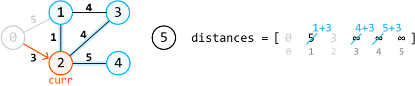
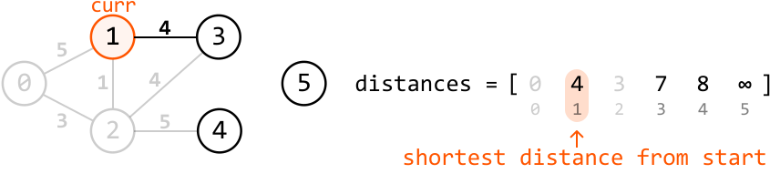
![Image represents a weighted graph displayed alongside a distance array. The graph consists of six nodes, numbered 0 through 5, connected by weighted edges. Node 0 connects to node 1 (weight 5) and node 2 (weight 3). Node 1 connects to node 2 (weight 1), node 3 (weight 4), and node 0 (weight 5). Node 2 connects to node 4 (weight 5) and node 3 (weight 4). Node 3 connects to node 1 (weight 4). Node 4 and node 5 are not connected to any other nodes in the graph. To the right of the graph, a Python-style array named `distances` is shown, containing values [0, 4, 3, 7, 8, ∞]. The numbers below the array (0, 1, 2, 3, 4, 5) correspond to the node indices, indicating that the distance from node 0 to node 0 is 0, to node 1 is 4, to node 2 is 3, to node 3 is 7, to node 4 is 8, and to node 5 is infinity (∞). The array represents the shortest path distances from node 0 to all other nodes in the graph.](images/img_21dc244623c4.svg)
![Image represents a Python list assignment. The variable `distances` is assigned a list containing six numerical values: `[0, 4, 3, 7, 8, -1]`. These values are enclosed within square brackets `[]`, indicating a list data structure. Below the list, smaller numbers `0, 1, 2, 3, 4, 5` are displayed, acting as indices representing the position of each element within the `distances` list. The index 0 corresponds to the value 0, index 1 to the value 4, and so on, with index 5 corresponding to the value -1. There is no explicit flow of information depicted; the image simply shows the assignment of values to the list variable.](images/img_5d0729220ec8.svg)
![Image represents a visualization of Dijkstra's algorithm's initial state. On the left, a weighted directed graph is shown with three nodes labeled 0, 1, and 2. Node 0 is marked as 'start'. Edges connect node 0 to node 1 with weight 6, and node 0 to node 2 with weight 3. Node 1 connects to node 2 with weight 1. Below the graph, a distances array is shown, initialized as [0, ∞, ∞], representing the initial distances from the start node (0) to each node (0, 1, and 2 respectively, where ∞ signifies infinity). On the right, a min-heap data structure is depicted, currently containing only node 0 with a value of 0, indicated by 'min: 0:0'. The min-heap is used to efficiently select the node with the smallest distance from the start node during the algorithm's execution. The overall image illustrates the setup before the algorithm begins iterating and updating distances.](images/img_daf7506aa973.svg)
![Image represents a step-by-step illustration of Dijkstra's algorithm using a min-heap. The left side shows the initial state: a graph with three nodes (0, 1, 2), where node 0 (labeled 'curr' and colored orange) is the current node with a distance of 0. Edges are weighted (6, 1, 3). A min-heap is shown alongside, containing the initial distances: node 0 at distance 0, and nodes 1 and 2 at infinity (∞). An arrow indicates that node 0 (with distance 0) is extracted from the min-heap, updating `curr_dist` to 0 and `curr_node` to 0. The right side depicts the state after updating the distances of node 0's neighbors. Node 1 and 2 are now colored cyan, reflecting their updated status. The distances to nodes 1 and 2 are updated to 6 and 3 respectively, reflected in the updated min-heap (6:1 and 3:2) and the `distances` array [0, 6, 3]. The arrow between the left and right sides signifies the transition between these states.](images/img_fc7f0543c5e9.svg)
![Image represents a step-by-step illustration of Dijkstra's algorithm, focusing on updating distances in a graph. The left side shows the initial state: a graph with nodes 0, 1, and 2, where node 2 (colored orange and labeled 'curr') is the current node being processed. Edges are labeled with their weights (6, 1, 3). A min-heap data structure is shown, containing node 1 with a distance of 6 and node 2 with a distance of 3 (indicated as 'min: 3:2'). The current distance to node 2 ('curr_dist') is 3, and an array 'distances' = [0, 6, 3] represents the shortest distances from node 0 to nodes 0, 1, and 2 respectively. An arrow points from the min-heap's '3:2' element to 'curr_dist = 3' and 'curr_node = 2', indicating the extraction of the current node and its distance from the heap. The right side depicts the state after updating the distances of node 2's neighbors. Node 1 is now colored light blue, reflecting its updated status. The min-heap now contains node 1 with a distance of 4 (1+3, shown as 'min: 1+3:1') and node 2 with a distance of 6. The 'distances' array is updated to [0, 4, 3], showing the new shortest distance to node 1. A large arrow separates the before and after states, illustrating the transition.](images/img_b5c978706a6c.svg)
![Image represents a step-by-step illustration of Dijkstra's algorithm. The left side shows the initial state: a graph with three nodes (0, 1, 2) connected by weighted edges (6, 1, 3), with node 1 highlighted as 'curr' (current node) in orange. Node 1 has a 'curr_dist' of 4. A min-heap data structure is shown, containing the element '6:1', indicating a distance of 6 to node 1. Below, a 'distances' array [0, 4, 3] represents the shortest distances found so far from a source node (not shown) to nodes 0, 1, and 2 respectively. A large arrow points to the right, indicating a transition. The right side depicts the state after processing node 1: the min-heap now contains '6:1', reflecting the updated distances. The 'distances' array is updated to [0, 4, 3], showing that the distances to nodes 0, 1, and 2 have been updated. The text ' (no unvisited neighbors)' indicates that all neighbors of the current node have been processed. The overall image demonstrates how Dijkstra's algorithm iteratively selects the node with the minimum distance from the min-heap, updates the distances of its neighbors, and repeats until all nodes are processed.](images/img_2144dfcdb35e.svg)
![Image represents a step in a graph traversal algorithm, likely Dijkstra's algorithm. The left side shows a weighted graph with three nodes (0, 1, and 2) and their connecting edges labeled with weights (6, 1, and 3). Node 1 is highlighted in orange and labeled 'curr,' indicating it's the currently selected node. A red curved arrow points to node 1, labeled 'previously visited,' suggesting a process of iteratively visiting nodes. Below the graph, 'curr_dist = 6' shows the current distance from the source node to node 1, and 'distances = [0 4 3]' represents an array storing the shortest distances from the source to each node (0, 1, and 2 respectively). The right side depicts a min-heap data structure labeled 'min_heap,' containing the element '6:1' (distance:node), signifying that node 1 with a distance of 6 is the element with the minimum distance currently in the heap. An orange arrow points from this element in the min-heap to 'curr_dist = 6' and 'curr_node = 1,' indicating that the node and its distance are extracted from the min-heap for processing. The overall image illustrates the process of selecting the node with the minimum distance from a min-heap and updating relevant variables.](images/img_b62436fc2237.svg)
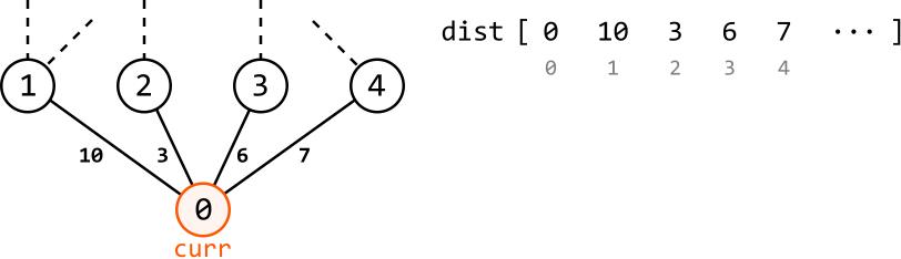
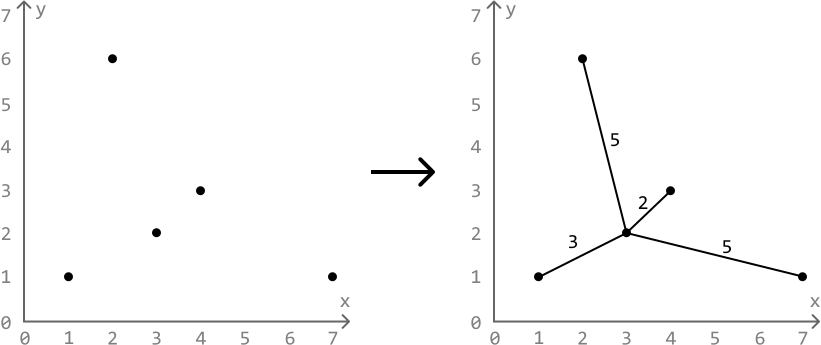
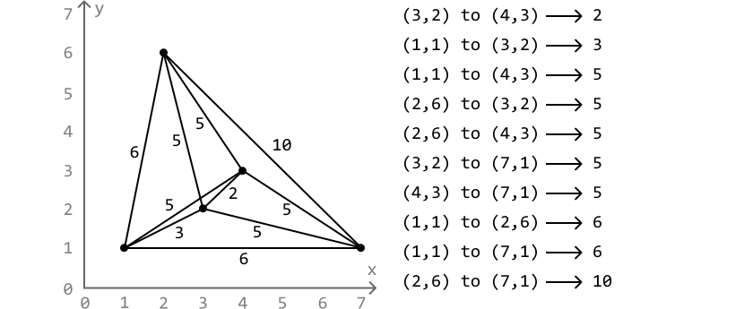
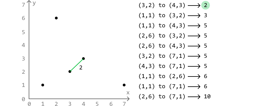
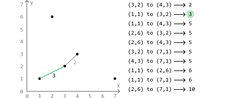
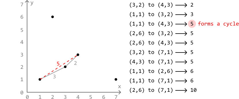
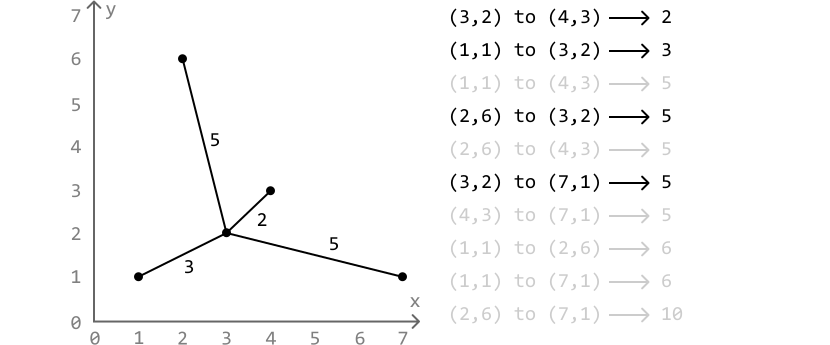
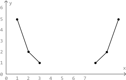
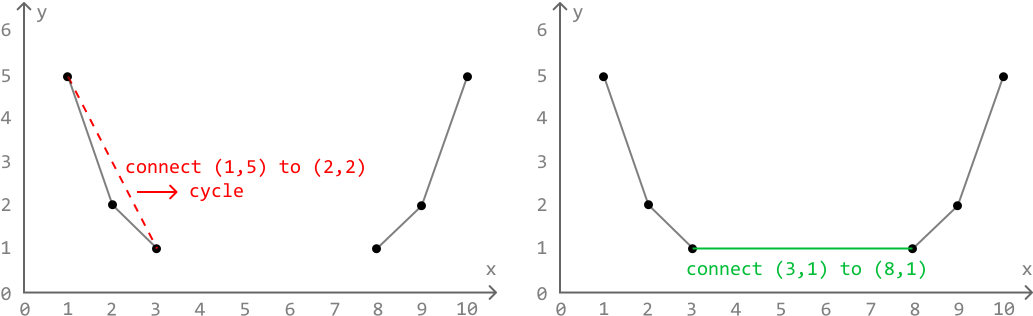
![Image represents a tree-like diagram illustrating a recursive algorithm, likely for generating permutations. The top row shows three initial states, each represented as '[], used = {}', indicating an empty permutation list and an empty set of used numbers. The input `nums = [4 5 6]` is defined at the top. From each initial state, a number is chosen (indicated by 'choose 4', 'choose 5', 'choose 6' in peach-colored boxes), represented by a downward-pointing arrow. This chosen number is appended to the permutation list, and added to the `used` set. The next level shows the updated state, for example '[4], used = {4}'. This process repeats recursively; each node represents a state with a partially built permutation and a set of used numbers. The arrows depict the flow of the algorithm, branching out as each number is chosen. The final state, '[4,5,6], used = {4,5,6}', is reached in the bottom-right branch, resulting in the message 'one permutation found!' in green, indicating a successful permutation generation. The diagram visually demonstrates the backtracking nature of the algorithm, as each branch explores a different permutation possibility.](images/img_d941f46b43e8.svg)
![Image represents a directed acyclic graph illustrating a backtracking algorithm, likely for a problem involving selecting elements from a set. The graph shows a sequence of states, each represented by a node labeled with a list `[]` indicating the selected elements and a set `{ }` labeled `used` showing the elements already considered. The top node `[], used = {}` represents the initial state with no elements selected. An arrow points downwards to `[4], used = {4}`, indicating that element 4 has been selected. Another downward arrow connects this to `[4,5], used = {4,5}`, showing that element 5 has subsequently been selected. A final downward arrow leads to `[4,5,6]`, suggesting element 6 was added. A light-blue box labeled 'backtrack: remove 6' and an upward arrow connects `[4,5,6]` to `[4,5]`, demonstrating a backtracking step where element 6 is removed to explore alternative solutions. The graph visually depicts the exploration of different combinations by adding and removing elements, a common characteristic of backtracking algorithms.](images/img_2b74e2bdb164.svg)
![Image represents a state diagram illustrating a backtracking algorithm, likely for a problem involving selecting elements from a set. The diagram shows a directed acyclic graph with nodes representing states and edges representing transitions. Each node is labeled with a list (representing a subset of elements selected so far) and a set named 'used' indicating which elements are already included in the subset. The top node, '[ ], used = {}', represents the initial state with no elements selected. A downward arrow connects this to '[4], used = {4}', indicating the selection of element 4. Another downward arrow leads to '[4, 5]', showing the subsequent selection of element 5. A further downward arrow connects to '[4, 5, 6]', suggesting the addition of element 6. Crucially, a light-blue box labeled 'backtrack: remove 5' and an upward arrow connects '[4, 5]' to '[4], used = {4}', demonstrating a backtracking step where element 5 is removed to explore alternative selections. The arrows indicate the flow of the algorithm, showing how it explores different combinations by adding and removing elements.](images/img_991d6be15b70.svg)
![Image represents a state-transition diagram illustrating a backtracking algorithm, likely for finding combinations or permutations. The diagram shows a tree-like structure where each node represents a state defined by a list (in square brackets) representing a partially built combination and a set (within curly braces) labeled 'used' tracking the elements already included. The root node is `[], used = {}`, indicating an empty initial combination and no used elements. A downward arrow signifies the addition of an element to the combination. From the root, a black arrow points to `[4], used = {4}`, showing the selection of element 4. From this node, two downward arrows branch to `[4,5]` and `[4,6], used = {4,6}`, representing the addition of 5 and 6 respectively, updating the 'used' set. A light-blue upward arrow connects `[4,5]` to `[4,5,6]`, suggesting a further addition of 6 (though this branch isn't fully explored). A rectangular box labeled 'choose 6' highlights the decision point where 6 is considered for addition to the combination. The overall structure demonstrates the exploration of different combinations by adding elements and backtracking when necessary, as indicated by the upward arrows.](images/img_66e3244d7bcf.svg)
![Image represents a tree-like diagram illustrating a backtracking algorithm for generating permutations. The root node is `[], used = {}`, indicating an empty initial set and an empty set of used numbers. A downward-pointing arrow connects this to the node `[4], used = {4}`, showing the selection of 4 as the first element. From this node, two branches extend downwards, representing the choices for the second element: `[4,5]` and `[4,6]`, with `used = {4,6}` indicating that 4 and 6 have been used. A light-blue upward-pointing arrow connects `[4,5]` to `[4,5,6]`, showing the addition of 6 as the third element. Similarly, a downward-pointing arrow from `[4,6]` leads to `[4,6,5]`. The text 'choose 5' highlights the selection of 5 in the lower branch. Finally, `[4,5,6]` and `[4,6,5]` represent complete permutations, with `used = {4,6,5}` indicating all used numbers, and the text 'found another permutation!' confirms the successful generation of a permutation. The diagram visually demonstrates the recursive exploration of possibilities and the backtracking process when a choice leads to a dead end.](images/img_abc773738f71.svg)
![Image represents a tree-like structure illustrating the permutations of the set {4, 5, 6}. The root node, at the top, is an empty set represented by `[]`. From this root, three branches descend, each representing a single element from the set: [4], [5], and [6]. Each of these nodes then branches further, adding one more element from the remaining set. For example, [4] branches into [4, 5] and [4, 6], representing the two possible ways to add one element from {5, 6} to the set {4}. This pattern continues until the bottom level, where each leaf node represents a complete permutation of the original set {4, 5, 6}, shown as ordered lists within square brackets: [4, 5, 6], [4, 6, 5], [5, 4, 6], [5, 6, 4], [6, 4, 5], and [6, 5, 4]. Arrows indicate the flow of information, showing how each permutation is built up sequentially from the root node.](images/img_a2d694988908.svg)

![Image represents a diagram illustrating an inclusive and exclusive range operation. A central node, labeled `[]`, represents the input range. From this central node, two lines extend to the left and right. The left line, labeled `incl. 4` in cyan, points to a node labeled `[4]`, indicating that the number 4 is included in the resulting range. Conversely, the right line, labeled `excl. 4` in orange, points to a node labeled `[]`, signifying that the number 4 is excluded from the resulting range on that side. The arrows indicate the direction of the range operation, showing how the input range is processed to produce two distinct output ranges based on inclusion or exclusion of the value 4.](images/img_9341661dbb76.svg)
![Image represents a binary tree structure illustrating a coding pattern. The root node, at the top, is represented by `[]`, indicating an empty array or list. This root node branches into two child nodes, also represented by `[]`. Each of these child nodes further branches into two more nodes. The left branches from the root and its child node are labeled `incl.5` in cyan, signifying the inclusion of the number 5. The right branches are labeled `excl.5` in orange, indicating the exclusion of 5. The leaf nodes at the bottom represent the resulting arrays after applying these inclusion/exclusion operations. Specifically, the leftmost leaf node shows `[4, 5]`, resulting from including 5 in the initial array `[4]`. The next leaf node is `[4]`, showing the result of excluding 5 from `[4]`. Similarly, on the right side, `[5]` represents including 5 in an initial empty array `[]`, and the final leaf node `[]` shows the result of excluding 5 from an empty array. The arrows indicate the flow of data and the operations performed at each node.](images/img_6f2c9b7d0528.svg)
![Image represents a binary tree illustrating a recursive algorithm, likely demonstrating subset generation or a similar combinatorial problem. The root node is an empty array `[]`. This root branches into two nodes: `[4]` and `[]`. Each subsequent node represents a subset. Each node with a numerical array splits into two child nodes: one where the number 6 is included (`incl. 6` in cyan), and one where it's excluded (`excl. 6` in orange). This pattern repeats down the tree. The leaf nodes show the final subsets generated: `[4,5,6]`, `[4,5]`, `[4,6]`, `[4]`, `[5,6]`, `[5]`, `[6]`, and `[]`. The arrows indicate the flow of the algorithm, showing how each subset is derived from its parent by either including or excluding the number 6.](images/img_2decd870432a.svg)
![Image represents a recursive tree structure illustrating a coding pattern, likely for generating subsets of a given array. The left side shows an iterative process, with boxes labeled 'i = 0', 'i = 1', 'i = 2', and 'i = 3' representing iterations, each accompanied by the array `nums` which is initially `[4, 5, 6]` and shrinks with each iteration. Arrows indicate the progression through the iterations. The main part of the image is a binary tree. Each node represents a subset of `nums`. The top node is an empty array `[]`. Each subsequent level branches into two nodes: one labeled 'incl nums[i]' (in cyan) representing the inclusion of the current element `nums[i]` in the subset, and the other labeled 'excl nums[i]' (in orange) representing its exclusion. The branches connect nodes, showing how subsets are built recursively by either including or excluding each element. The leaf nodes at the bottom show all possible subsets of the original array `[4, 5, 6]`, ranging from the empty set `[]` to the full set `[4, 5, 6]`.](images/img_83db045c6692.svg)
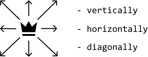
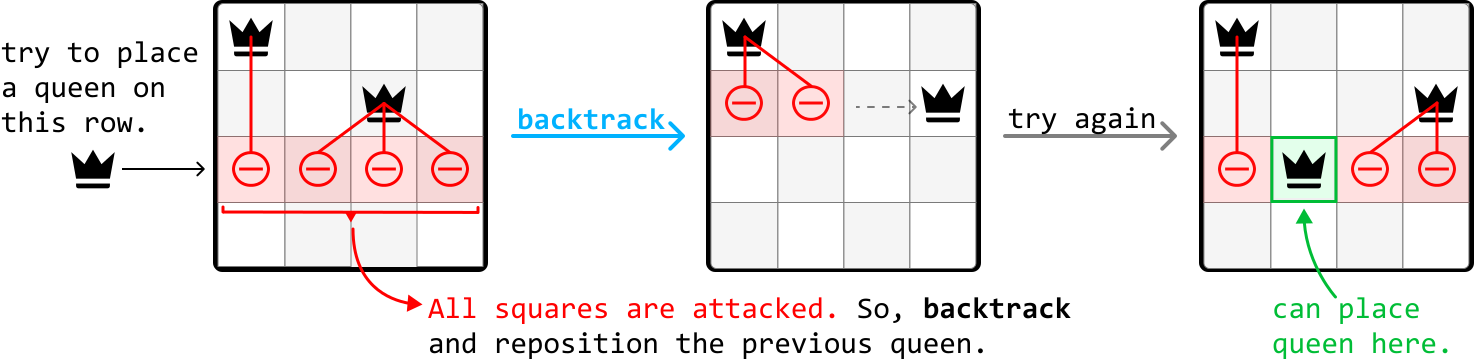
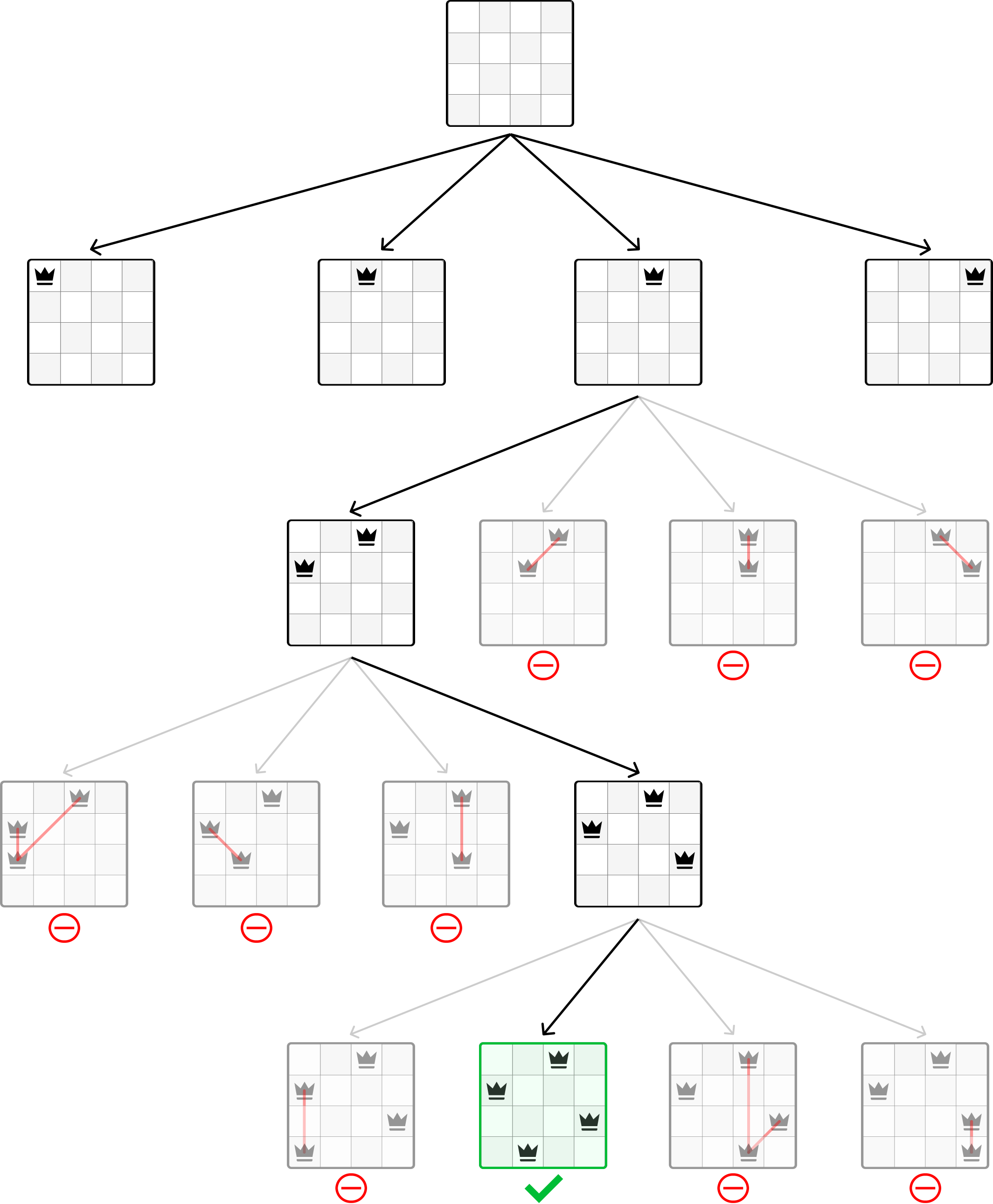
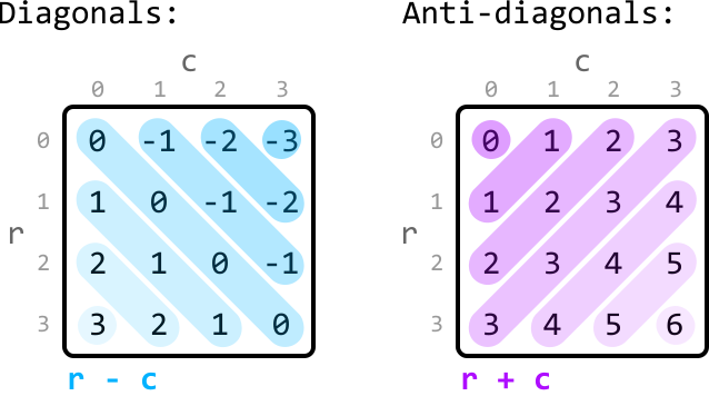

![Image represents a decision tree illustrating a choice between three options. A central node, labeled '[]' (representing the decision point), branches out to three leaf nodes labeled '[1]', '[2]', and '[3]'. Each branch is labeled with the text 'choose' in orange, followed by a number (1, 2, or 3) indicating the selected option. Arrows point from the central node to each leaf node, signifying the flow of control based on the choice made. The numbers 1, 2, and 3 represent the three possible outcomes or paths resulting from the decision at the central node. The square brackets around the leaf node labels might indicate an array or list structure in a programming context.](images/img_9a00c676afaa.svg)
![Image represents a tree-like structure illustrating a recursive algorithm, possibly for finding combinations. The root node is an empty array `[]`. From the root, three branches extend, labeled with orange numbers 1, 2, and 3, respectively, pointing to nodes `[1]`, `[2]`, and `[3]`. Each of these nodes further branches into three sub-nodes, again labeled 1, 2, and 3, resulting in leaf nodes representing two-element arrays like `[1,1]`, `[1,2]`, `[1,3]`, etc. Each leaf node displays the sum of its elements. A green checkmark indicates that the sum equals 4, while a red 'X' signifies a sum greater than 4. Dashed lines connect the leaf nodes to unseen underlying elements, suggesting further recursion or exploration of possibilities. The orange numbers on the branches seem to represent the values being added to the array at each level.](images/img_1e2467d6288a.svg)
![Image represents a tree-like structure illustrating a coding pattern, possibly related to recursion or tree traversal. The root node is labeled `[]`, representing an empty array or the starting point. From the root, three branches descend, each labeled `[1]`, `[2]`, and `[3]`, respectively. Each of these nodes further branches into three child nodes, representing arrays with two elements. For example, `[1]` branches into `[1,1]`, `[1,2]`, and `[1,3]`. The nodes `[2,1]`, `[3,1]`, and `[3,2]` are highlighted in a peach/light orange color. Curved arrows connect certain pairs of these leaf nodes, labeled 'duplicate' in a corresponding color (peach/light orange for the peach/light orange nodes, and gold for the other nodes). These arrows indicate that the connected nodes represent duplicate or redundant data structures within the overall pattern. The structure visually demonstrates how different combinations of elements can arise from a recursive or iterative process, and highlights the identification and handling of duplicate results.](images/img_890cb84bb3bd.svg)
![Image represents a tree-like structure illustrating a recursive algorithm, possibly for finding subsets of an array `nums = [1, 2, 3]` that sum to 4. The root node is `[], start_index = 0`, representing an empty subset and a starting index of 0. From the root, three branches extend, each representing a subset starting with one of the elements from `nums`. Each node shows the current subset (e.g., `[1]`, `[2]`, `[3]`) and its `start_index`. These nodes further branch, recursively adding subsequent elements from `nums` (starting from the `start_index`). The leaf nodes display the final subsets (e.g., `[1, 1]`, `[1, 2]`, `[1, 3]`, etc.). Each leaf node is labeled with the sum of its elements; those summing to 4 are marked in green (`sum == 4`), while those exceeding 4 are marked in red (`sum > 4`). The arrows indicate the flow of the algorithm, showing how subsets are built recursively. The gray arrows represent paths that are not explored further because they exceed the target sum.](images/img_eaaa41b84ba8.svg)
![Image represents a decision tree illustrating a recursive process, possibly for finding a subset of numbers that sums to a target value. The root node shows an empty array `[]` with a `target` value of 4. Three branches emanate from this root, each labeled with 'choose' followed by a number (1, 2, or 3), representing the selection of an element (implicitly from a larger set not shown). Each branch leads to a child node. These child nodes display an array containing the chosen element (e.g., `[1]`, `[2]`, `[3]`) and an updated `target` value, calculated by subtracting the chosen element from the previous target (e.g., 4-1=3, 4-2=2, 4-3=1). The updated `target` value suggests a recursive continuation of the process, where the algorithm would continue to choose elements until the target becomes zero, implying a solution has been found, or becomes negative, indicating no solution exists with the chosen path. The structure visually depicts the exploration of different solution paths through recursive choices.](images/img_d6d6725ffe36.svg)
![Image represents a decision tree illustrating a recursive algorithm, likely for finding combinations that sum to a target value. The root node is `[]`, target = 4, representing an empty initial set and a target sum of 4. From this root, three branches descend, labeled 1, 2, and 3, representing the addition of those numbers to the set. Each subsequent node shows the current set (e.g., `[1,1]`) and the remaining target value (e.g., `target = 3-1 = 2`), calculated by subtracting the added number from the previous target. The tree continues recursively until the target becomes 0 (e.g., `[1,3]`, `[2,2]`), at which point a green arrow indicates that the combination is added to the result and the branch terminates. If the target becomes negative (e.g., `[2,3]`, `[3,3]`), a red arrow points to 'stop,' signifying that this branch does not yield a solution. The orange numbers on the branches indicate the number being added at each step. The algorithm explores all possible combinations by systematically adding numbers from 1 to 3 until either the target is reached or it becomes negative.](images/img_9ee7155140b8.svg)


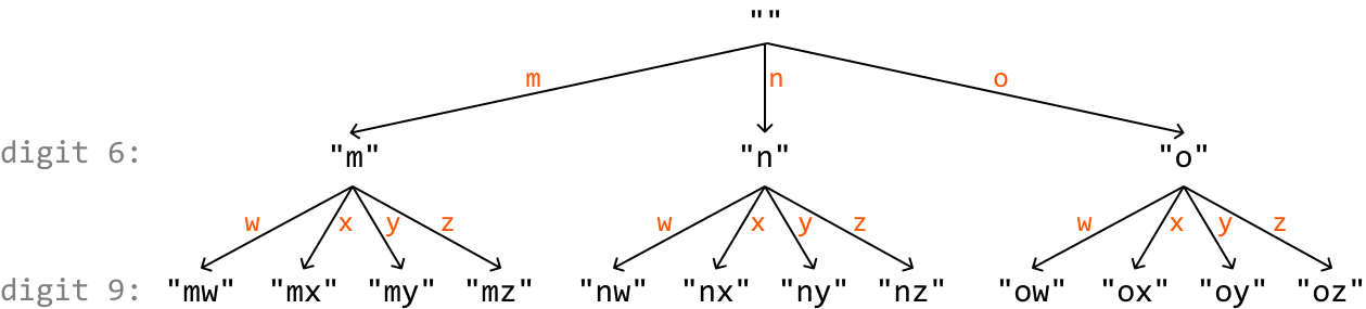
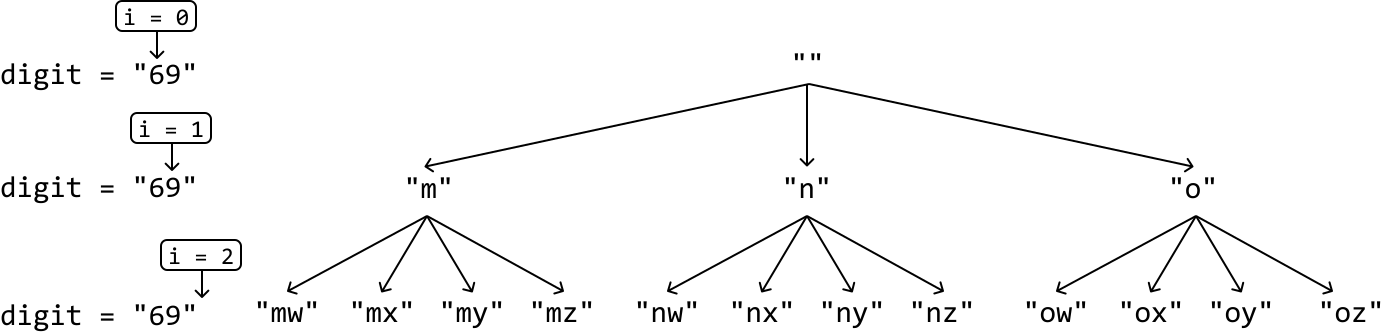
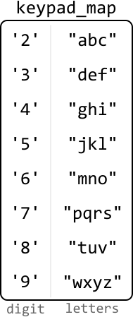
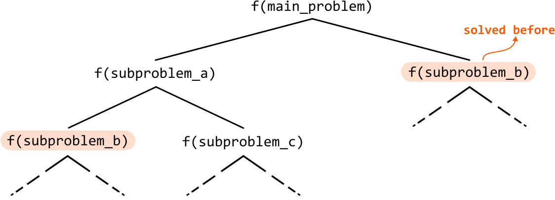
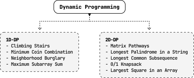
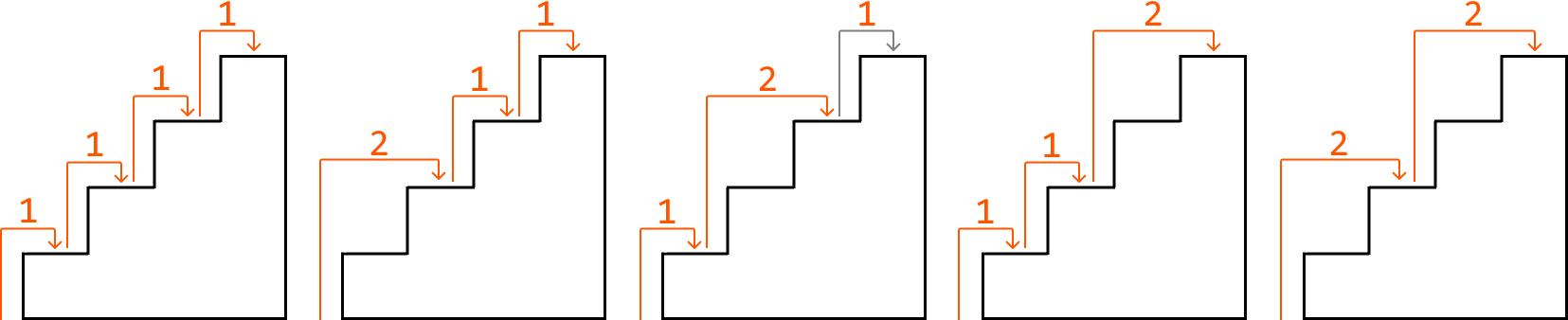
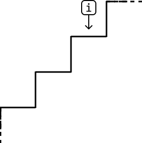
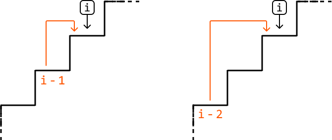
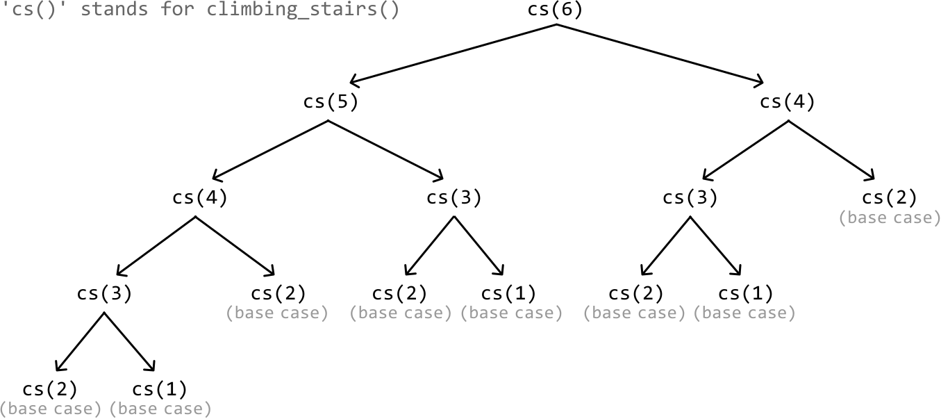
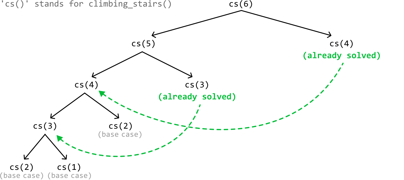
![Image represents a simple input for a coding problem, likely related to searching or summing within an array. The input consists of two parts presented linearly. The first part is an integer array represented by `[1 2 3]`, enclosed in square brackets, with the integers 1, 2, and 3 separated by spaces. This array is followed by a comma and a space, separating it from the second part. The second part specifies a target value, denoted by `target = 5`, indicating that the algorithm should search for, or use, the value 5 in relation to the array. There are no URLs or parameters present; the image solely displays the input data. The arrangement suggests that the array `[1 2 3]` and the target value `5` are independent inputs to a function or algorithm.](images/img_132aca7c76eb.svg)
![Image represents a simple data flow diagram illustrating a change in a parameter. The diagram begins with the word 'use' positioned above a downward-pointing arrow, indicating the input or application of a parameter. The arrow points to the input data: an array `[1 2 3]` and a parameter labeled `target = 5`. A solid arrow then connects this input to a new state, where the array remains the same, `[1 2 3]`, but the `target` parameter has changed to `target = 2`. The diagram visually depicts a process where the array remains constant, while the `target` parameter is modified from 5 to 2, suggesting a change in the input or a transformation within a system.](images/img_213ba56afbf1.svg)

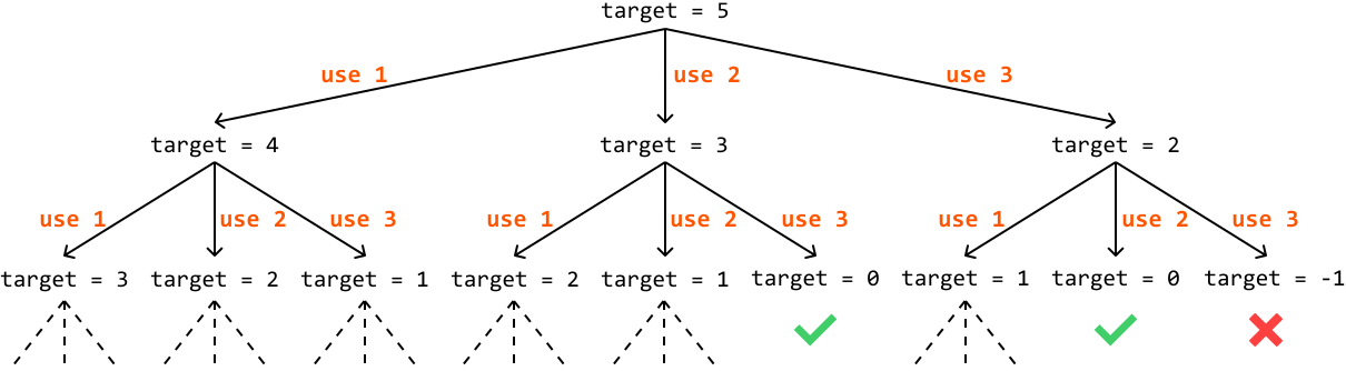
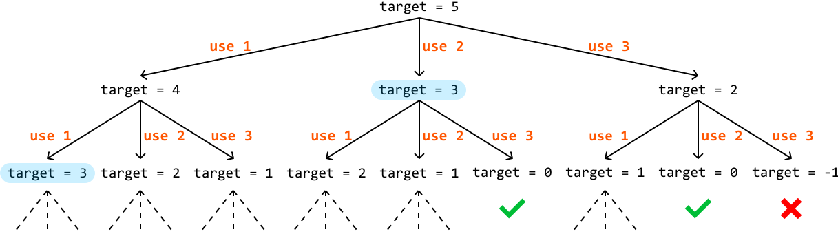
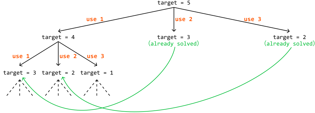

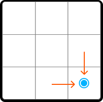
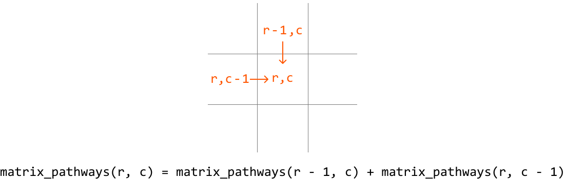
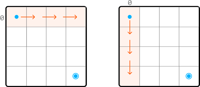
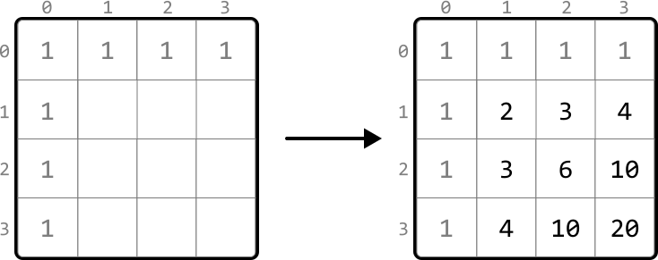
![Image represents a 2x2 grid illustrating a dynamic programming approach, likely for a problem involving a 2D array or matrix. The grid is divided into four quadrants, each representing a cell in the DP table. The top-right quadrant is labeled `dp[r-1][c]`, representing the value at row `r-1` and column `c`. The bottom-left quadrant is labeled `dp[r][c-1]`, representing the value at row `r` and column `c-1`. The bottom-right quadrant is labeled `dp[r][c]`, representing the value at row `r` and column `c`. A downward-pointing arrow connects `dp[r-1][c]` to `dp[r][c]`, indicating a dependency; the value of `dp[r][c]` is calculated using the value of `dp[r-1][c]`. A rightward-pointing arrow connects `dp[r][c-1]` to `dp[r][c]`, indicating another dependency; the value of `dp[r][c]` also depends on the value of `dp[r][c-1]`. This suggests a recursive or iterative approach where the value of each cell is computed based on the values of its top and left neighbors.](images/img_d10cb0476fa5.svg)
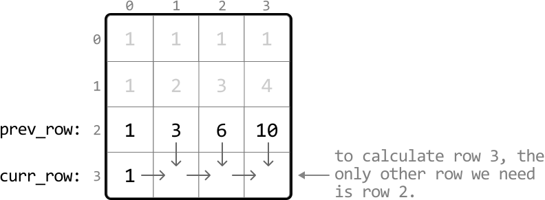
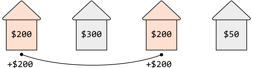
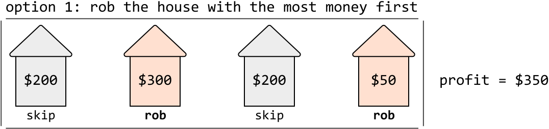
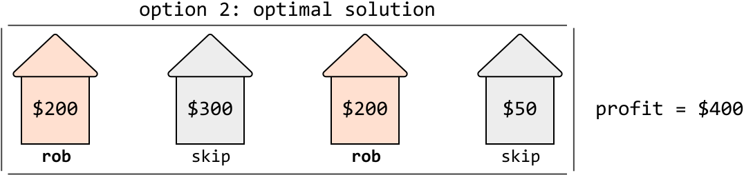
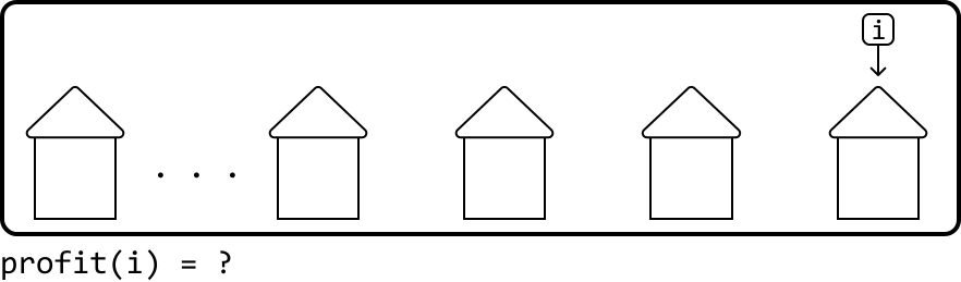
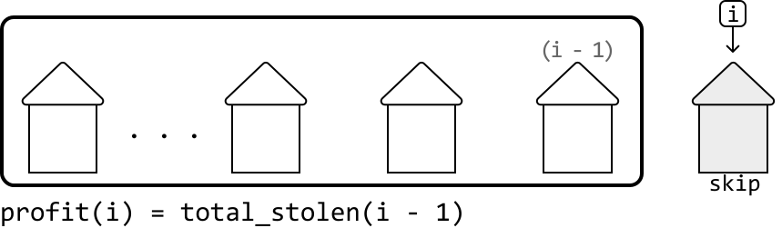
![Image represents a diagram illustrating a dynamic programming approach to solving the 'House Robber II' problem. A rectangular box contains a sequence of house icons representing houses in a circular street; an ellipsis (...) indicates that there are more houses not explicitly shown. Three houses are visible within the box, labeled (i-2), (i-1), and implicitly (i) which is the current house being considered. Outside the box, two additional houses are shown. The house labeled (i-1) is light gray, labeled 'skip,' indicating that this house is not robbed in the current iteration. The house to its right is peach-colored, labeled 'rob,' representing the current house being robbed. An arrow descends from a small square containing an 'i' symbol, pointing to the 'rob' house, suggesting an iterative process. The equation `profit(i) = houses[i] + total_stolen(i - 2)` below the diagram shows the recursive relationship: the profit from robbing house `i` is the value of house `i` plus the total stolen from houses up to (but not including) house `i-1`. The diagram visually demonstrates the decision-making process at each step, choosing between robbing the current house (`rob`) or skipping it (`skip`) based on maximizing the total profit, considering the constraint of not robbing adjacent houses.](images/img_4762b80c767f.svg)



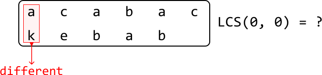



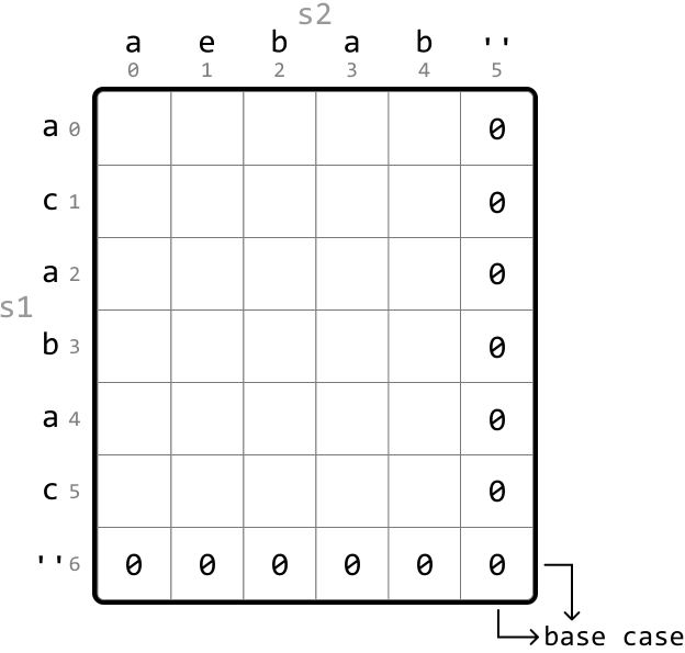
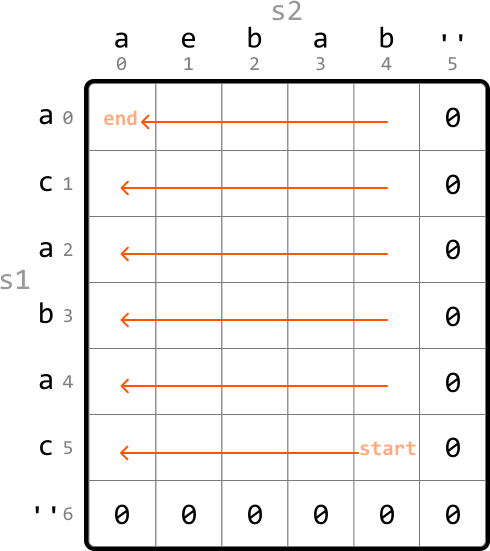
![Image represents a 2x2 grid illustrating a dynamic programming (DP) state transition. The grid is divided into four cells, each representing a subproblem's solution denoted by `dp[i][j]`, `dp[i][j+1]`, `dp[i+1][j]`, and `dp[i+1][j+1]`, where `i` and `j` are indices. The shaded cells, `dp[i+1][j]` and `dp[i+1][j+1]`, represent solutions to subproblems with incremented indices. Grey arrows indicate the flow of information, showing that the solution to the current subproblem `dp[i][j]` is derived from the solutions of the subproblems `dp[i][j+1]` and `dp[i+1][j]`. Specifically, `dp[i][j]` receives input from `dp[i][j+1]` and `dp[i+1][j]`, suggesting a recursive relationship where the optimal solution for `dp[i][j]` depends on the optimal solutions of its neighboring subproblems to the right (`dp[i][j+1]`) and below (`dp[i+1][j]`). The arrow from `dp[i+1][j+1]` to `dp[i][j]` is less prominent, suggesting a less direct or conditional dependency.](images/img_96a4a5912ef2.svg)
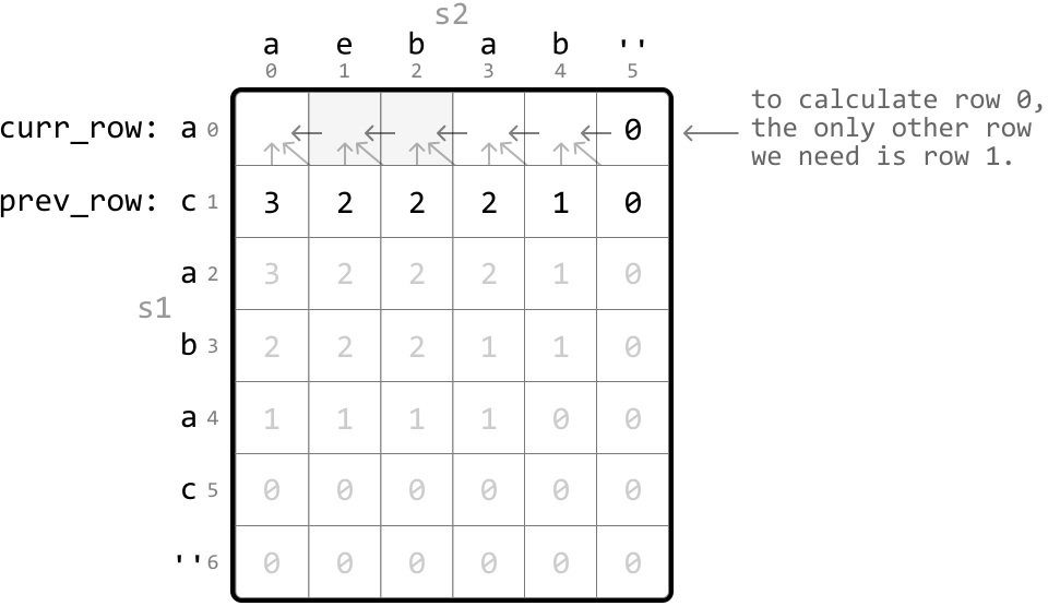
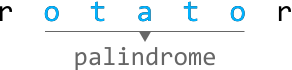
![Image represents a visual explanation of a palindrome-checking algorithm. The core element is a string 'rotor' displayed in light blue, representing the input string 's'. Two orange boxes labeled 'i' and 'j' act as pointers, initially pointing to the first ('r') and last ('r') characters of the string, respectively. Dashed grey arrows indicate the flow of comparison: 'i' points downwards to the 'r' at the beginning, and 'j' points downwards to the 'r' at the end. Above the string, 's[i] == s[j]' in orange text signifies the comparison of characters at indices 'i' and 'j'. If the characters are equal (as they are in this case), the algorithm proceeds. Below the string, 's[i + 1 : j - 1]' in orange and black text indicates the substring remaining after the initial comparison, which is 'ota to'. This substring is declared to be a palindrome, implying that the algorithm recursively checks this substring for the same condition until either a mismatch is found or the substring becomes empty, confirming the original string's palindrome status.](images/img_f1e865692f3d.svg)


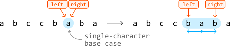
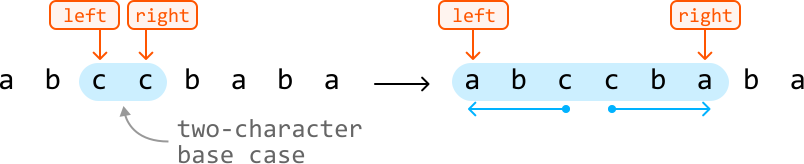
![Image represents a one-dimensional array or list of integers. The array is enclosed in square brackets `[` and `]`. The integers within the array are `3`, `1`, `-6`, `2`, `-1`, `4`, and `-9`, each separated by a space. Below each integer, in a lighter gray font, are the corresponding indices of the array, starting from 0 and incrementing sequentially: `0`, `1`, `2`, `3`, `4`, `5`, and `6`. There are no visible connections or information flow between the elements other than their sequential arrangement within the array structure, implicitly indicating that each integer is accessible via its index.](images/img_064ffe0e8570.svg)
![Image represents a visual depiction of an array and a variable update. An array `num` is shown, containing the integer elements [3, 1, -6, 2, -1, 4, -9], with each element's index displayed below it (0 through 6). A downward-pointing orange arrow labeled 'num' points to the first element of the array, the number 3, which is highlighted in a peach-colored circle. To the right, a dashed-line box shows the variable `curr_sum` being updated. The expression `curr_sum += 3` indicates that 3 is added to the current value of `curr_sum`, resulting in a new value of 3, as shown by `curr_sum = 3`. The diagram illustrates the process of accessing and using a specific element (the first element) from an array within a calculation.](images/img_1e69db8733b6.svg)
![Image represents a visual depiction of an array and an operation performed on it. A numerical array `[3, 1, -6, 2, -1, 4, -9]` is shown, with each element indexed from 0 to 6 below it. An orange arrow labeled 'num' points downwards to the element at index 1, which is the number 1, highlighting it as the current element being processed. To the right, a dashed-line box shows the operation being performed: `curr_sum += 1`, indicating that 1 is being added to a variable named `curr_sum`. Below this, `= 4` shows the resulting value of `curr_sum` after the addition. The diagram illustrates a step in an iterative process, likely summing the elements of the array, with the highlighted element contributing to the running sum.](images/img_770d5442f594.svg)
![Image represents a visual depiction of a step in an algorithm, likely involving array processing and sum calculation. A peach-colored highlighted section of an array `[3 1 -6 2 -1 4 -9]` is shown, with the element `-6` at index 2 indicated by an orange downward-pointing arrow labeled 'num'. This suggests that the algorithm is currently processing the element at index 2. To the right, a light gray box represents a variable named `curr_sum`. Inside this box, the calculation `curr_sum += -6` is shown, indicating that -6 is being added to the current value of `curr_sum`. Below this, `= -2` shows the resulting value of `curr_sum` after the addition. A rightward-pointing arrow labeled 'larger' connects to the `-2`, suggesting that this value is being compared or used to determine a 'larger' value in a subsequent step of the algorithm. The array indices are displayed below the array elements, ranging from 0 to 6.](images/img_2780e24d6913.svg)
![Image represents a step-by-step illustration of a coding pattern, likely related to finding the minimum value in an array. The top shows the word 'num' in orange, with a downward arrow pointing to a peach-colored circle containing '-6'. This circle is positioned within a larger array representation: `[3, 1, -6, 2, -1, 4, -9]`, with each element's index (0-6) displayed below it. The '-6' in the circle is highlighted, indicating the current element being processed. To the right, a dashed-line box displays 'curr_sum = -6', representing the current minimum sum found so far. An arrow labeled 'smaller' points from the right to the 'curr_sum' box, indicating that the value '-6' is being compared and potentially updated as the minimum. The overall diagram visually demonstrates the iterative process of comparing each element of the array to the current minimum, updating the minimum if a smaller value is encountered.](images/img_fb236dee6384.svg)
![Image represents a visual depiction of a coding pattern, likely illustrating a step within an algorithm. A peach-colored rectangular segment highlights a portion of a numerical array: `[3 1 -6 2 -1 4 -9]`, with indices 0 through 6 displayed below each element. An orange arrow labeled 'num' points downwards onto the highlighted segment, indicating that the variable 'num' is referencing or operating on this section of the array (specifically elements at indices 0, 1, 2, and 3). To the right, a dashed-line box represents a variable named 'curr_sum'. Inside this box, the expression 'curr_sum += 2' indicates that 2 is being added to the current value of 'curr_sum'. Below this, '= 0' shows the current value of 'curr_sum' is 0. A grey arrow points from the right to the 'curr_sum' box, labeled 'smaller', suggesting that the value of 'smaller' (not shown) is influencing or updating 'curr_sum'. The overall diagram suggests a process where a section of an array is being processed, potentially to find a minimum or maximum value, and a running sum ('curr_sum') is being updated based on this processing.](images/img_b5c6c383b176.svg)
![Image represents a snapshot of an algorithm's execution, likely demonstrating a coding pattern related to array traversal and sum calculation. A numerical array `[3, 1, -6, 2, -1, 4, -9]` is displayed, with each element indexed from 0 to 6. A light peach-colored circle highlights the element '2' at index 3, with an orange arrow labeled 'num' pointing to it, indicating the current element being processed. To the right, a dashed-line box displays 'curr_sum = 2', representing the current sum calculated so far. A rightward arrow connects this box to the word 'larger', suggesting that the algorithm is comparing the current sum with a larger value (not explicitly shown) as part of a larger process, possibly finding the largest contiguous subarray sum. The overall arrangement visually depicts a step-by-step process where the algorithm iterates through the array, updating the `curr_sum` and comparing it to find a larger value.](images/img_220e47969af8.svg)
![Image represents a step-by-step illustration of a coding pattern, likely for finding the maximum contiguous subarray sum. The left side shows an array `[3, 1, -6, 2, -1, 4, -9]` with indices 0 through 6 displayed below each element. An orange arrow labeled 'num' points to the element '2' at index 3 and '-1' at index 4, indicating the current element being processed. A peach-colored rectangle highlights these two elements. The right side shows a calculation box detailing the algorithm's logic. A curved arrow points from the text '(previous curr_sum value)' to the calculation box. Inside the box, the equation `curr_sum = max(curr_sum + num, num)` is shown, representing the update of the maximum sum so far. Below, a substitution with `curr_sum = 2` and `num = -1` is shown, resulting in `max(2 + (-1), -1)`, which simplifies to `max(1, -1) = 1`. This demonstrates how the algorithm updates the maximum sum based on the current element and the previous maximum sum.](images/img_67e58c54d4ea.svg)
![Image represents a visual explanation of a maximum subarray sum calculation. A numerical array `[3, 1, -6, 2, -1, 4, -9]` is shown, with indices 0 through 6 displayed below each element. A peach-colored rectangle highlights the element '2', '-1', and '4' within the array. An orange arrow labeled 'num' points downwards, indicating that the value '4' is currently being processed. To the right, a light gray box details the calculation: `curr_sum = max(curr_sum + num, num)`, where `curr_sum` represents the current maximum sum and `num` represents the current element (4). The calculation is broken down in subsequent lines: `= max(1 + 4, 4)` showing the substitution of values, and finally `= 5`, indicating that the current maximum sum is updated to 5. The diagram illustrates a step in an algorithm that iterates through the array, updating the maximum sum based on the current element and the running sum.](images/img_c05deb8617c1.svg)
![Image represents a visual explanation of a maximum subarray sum calculation. A numerical array `[3, 1, -6, 2, -1, 4, -9]` is shown, with each element indexed from 0 to 6. A peach-colored rectangle highlights the element at index 3, the number `2`, which is labeled with an orange arrow pointing to it as 'num'. To the right, a calculation is displayed showing the running maximum sum (`curr_sum`). The formula `curr_sum = max(curr_sum + num, num)` is presented, demonstrating how the current maximum sum is updated by taking the maximum between the current sum plus the current element (`num`) and the current element itself. The calculation is then shown step-by-step: `max(5 + (-9), -9)` which simplifies to `-4`, indicating that at this step, the maximum subarray sum is -4. The indices below the array visually correspond to the array elements.](images/img_1fff05f96ec9.svg)
![Image represents a numerical array depicted as `[3 1 -6 2 -1 4 -9]`, enclosed in square brackets. A peach-colored rectangle highlights the first four elements (3, 1, -6, 2) of this array. Beneath the array, numbers 0 through 6 are displayed, acting as indices corresponding to each element's position within the array. To the right of the array, the text 'sum = 0' is shown in orange, indicating that the sum of all elements within the array equals zero. There are no URLs or parameters present in the image; the image solely illustrates an array and its sum.](images/img_0f0cc3898116.svg)
![Image represents a numerical array depicted within square brackets `[]`, showing a sequence of numbers: 3, 1, -6, 2, -1, 4, -9. A light peach-colored rectangle highlights the sub-array [1, -6, 2]. Beneath the array, numbers 0 through 6 are displayed, acting as indices corresponding to each element's position within the array. To the right of the array, the text 'sum = -3' is shown in orange, indicating the sum of all the numbers in the array is -3. There is no explicit connection shown between the highlighted sub-array and the sum calculation; the highlighting simply draws attention to a specific portion of the array.](images/img_f4a48dad128f.svg)
![Image represents a numerical array depicted within square brackets `[]`, containing the elements 3, 1, -6, 2, -1, 4, and -9. Each element is positioned sequentially, with indices 0 through 6 displayed below them in gray. A peach-colored oval highlights the elements -6 and 2, suggesting a focus or operation on these specific values. To the right of the array, the text 'Sum = -4' is displayed in orange, indicating the sum of all elements within the array is -4. The arrangement visually demonstrates the calculation of the sum of the elements in the array, with the highlighted section possibly representing a sub-calculation or a specific part of the summation process.](images/img_a26f147e81d5.svg)
![Image represents a visual depiction of a maximum subarray sum algorithm. A numerical array `[3, 1, -6, 2, -1, 4, -9]` is shown, with each element's index displayed below it (0 through 6). The element at index 3, the number '2', is highlighted with a peach-colored circle. To the right, a green rectangular box displays the result 'sum = 2', indicating that the maximum contiguous subarray sum within the given array is 2. The word 'max' is written in green above the result box, clarifying that the displayed value represents the maximum sum. The highlighted '2' visually suggests that this element is part of, or possibly the maximum subarray itself, although the algorithm's exact steps aren't explicitly shown. The diagram focuses on presenting the input array and the final result of the maximum subarray sum calculation.](images/img_950f658879a0.svg)
![Image represents a visual depiction of a subproblem within a dynamic programming approach, likely to find the maximum subarray sum. A rectangular box contains a numerical array `[3, 1, -6, 2, -1, 4, -9]` with indices 0 through 6 displayed below each element. A small square labeled 'i' is positioned above the array, with a downward arrow indicating input to the array. To the right of the array, the text 'max_subarray(i) = ?' is displayed, posing a question about the maximum subarray sum up to index 'i'. The overall structure suggests an illustration of a single step in an algorithm where the input 'i' (likely representing an index) determines a subarray, and the question mark indicates the algorithm's goal of finding the maximum sum within that subarray.](images/img_d67173cb1963.svg)
![Image represents a visual depiction of a step in a dynamic programming algorithm, likely for finding the maximum sum subarray. A rectangular box displays an array of integers: [3, 1, -6, 2, -1, 4, -9], with indices 0 through 6 displayed below each element. A small square labeled 'i' points down to the element -9 at index 6, indicating the current index being processed. To the right, the expression `max_subarray(i - 1) + (-9)` is shown, illustrating the recursive or iterative step of the algorithm. This formula suggests that the maximum subarray sum ending at index `i` is calculated by adding the maximum subarray sum ending at the previous index (`i - 1`) to the value at the current index (`-9`). The arrow from 'i' to -9 visually connects the index to the element used in the calculation, demonstrating the flow of information within the algorithm. The peach-colored highlighting of -9 emphasizes its role in the current calculation step.](images/img_84aa5a12ace4.svg)
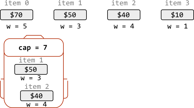

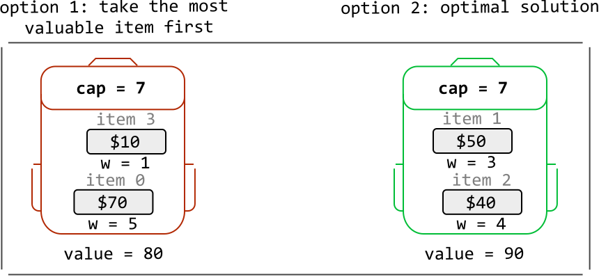
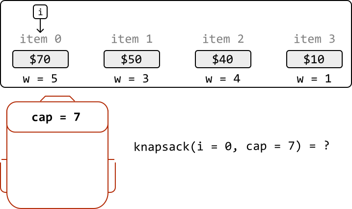
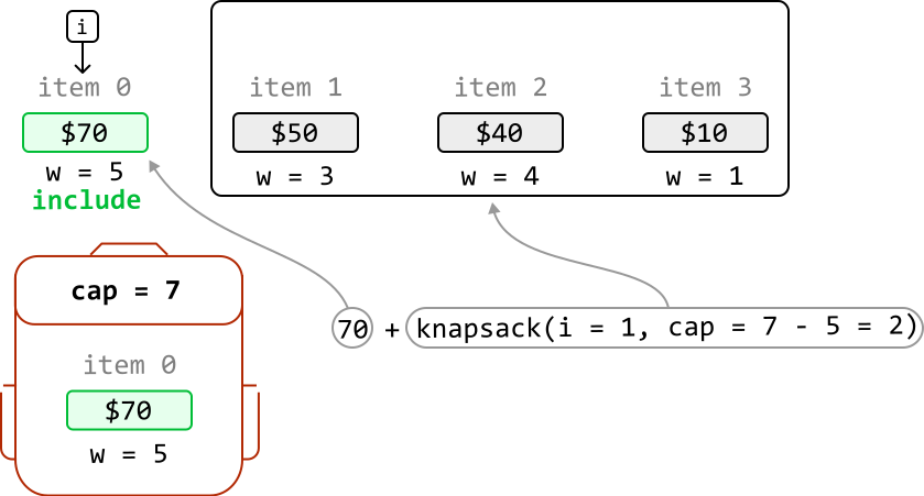
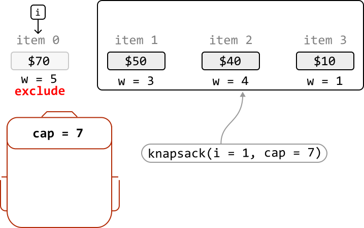
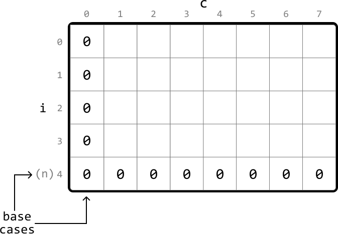
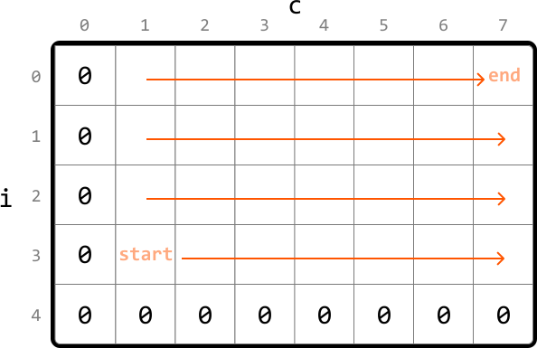
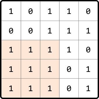
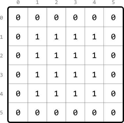
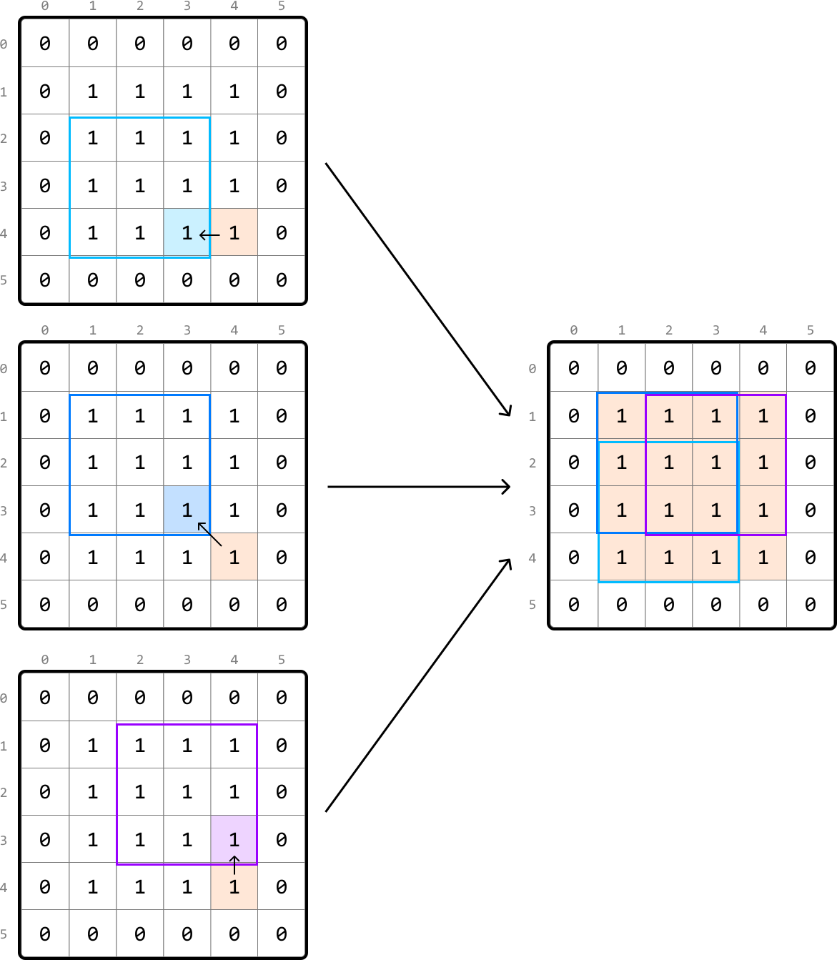
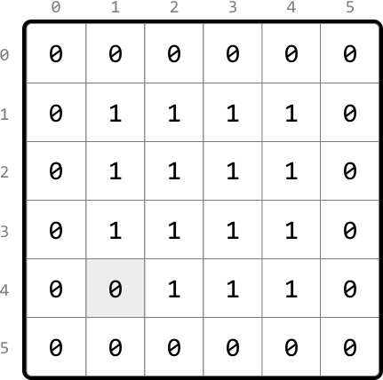
![Image represents a step-by-step visualization of a 2D array processing algorithm, likely demonstrating a sliding window or kernel operation. Three 6x6 matrices are shown, each representing a stage in the process. The matrices contain only 0s and 1s. In the first matrix, a 2x2 region (cells [3,2] to [4,3]) is highlighted with a light blue border. An arrow points from the cell [3,3] to [4,3], suggesting data movement or processing. The second matrix shows the light blue region shifted one position to the right, now encompassing cells [3,3] to [4,4], with a new light blue region. A similar arrow points from [3,4] to [4,4]. The third matrix shows a larger, 3x3 region (cells [1,2] to [3,4]) highlighted with a purple border, encompassing the previous light blue regions, suggesting an accumulation or aggregation of results. Arrows connect the matrices, indicating the sequential nature of the algorithm. The row and column indices (0-5) are labeled along the top and left side of each matrix, providing spatial context. The overall diagram illustrates a pattern of iterative processing across a 2D array, possibly for tasks like image filtering or feature extraction.](images/img_e6eae57d456c.svg)
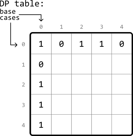
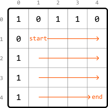
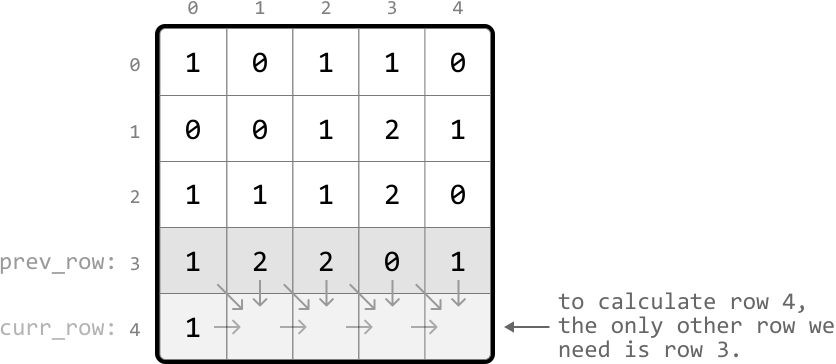
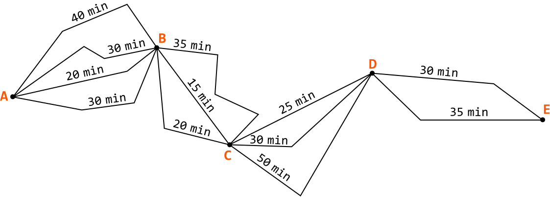
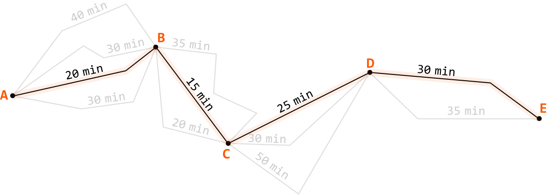
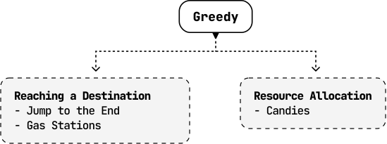
![Image represents a sequence of numbers, [3, 2, 0, 2, 5], depicted within square brackets. A green curved arrow originates from the number 3 at the beginning of the sequence and points to the number 2 near the middle. Another smaller green curved arrow originates from the same initial 2 and points to the number 5 at the end of the sequence. These arrows suggest a connection or flow of information, possibly indicating a relationship or operation between the numbers 3 and 2, and separately between the number 2 and 5. The arrangement implies a linear data structure, possibly an array or list, with the arrows highlighting specific elements and their interactions within the context of a coding pattern, likely illustrating a selection or traversal process.](images/img_8e6ad229892d.svg)
![Image represents two diagrams illustrating different scenarios of data flow or program execution. Each diagram shows a sequence of numbers, [2, 1, 0, 3], enclosed in square brackets. In both diagrams, a grey curved arrow points from the '0' to the text 'dead end,' indicating a termination point or a path that doesn't continue further. The key difference lies in the red arrows. In the first diagram, a single red curved arrow points from the '2' to the '0', suggesting a direct transition or flow from '2' to '0'. In the second diagram, two red curved arrows originate from the '2', one pointing to the '1' and the other to the '0', illustrating a branching or conditional flow where '2' can lead to either '1' or '0' before potentially reaching the 'dead end'. The diagrams likely depict different control flows or execution paths within a program, possibly highlighting the concept of a single path versus multiple paths, or a decision point in the algorithm.](images/img_7c2e492bf3fd.svg)
![Image represents a visual explanation of array traversal. A small square labeled 'i' points downwards with an arrow to an array `[3, 2, 0, 2, 5]`. Beneath the array, indices 0 through 4 are displayed. A curved orange arrow originates from the element at index 1 (value 2) and points to the element at index 3 (value 2). This arrow illustrates a jump in the array. The text below the array explains that this jump represents the 'furthest index we can jump to from i = i + nums[i]', indicating that the value at index `i` (in this case, 2) is added to `i` to determine the next index to visit. The formula `i + nums[i]` shows how the jump is calculated.](images/img_95891033ff4e.svg)
![Image represents a two-row array of numbers. The top row, enclosed in square brackets `[ ]`, displays the numbers 3, 2, 0, 2, and 5 in bold, black font, representing the main data set. Below this, a second row shows the indices 0, 1, 2, 3, and 4 in a lighter gray font, indicating the position or index of each corresponding element in the top row. The arrangement is linear, with each number in the top row directly above its corresponding index in the bottom row. No explicit connections or information flow is depicted beyond the implied positional relationship between the top and bottom rows.](images/img_1d41ce92c6bb.svg)
![The image represents a visual depiction of an array or list data structure. The main component is a numerical array `[3, 2, 0, 2, 5]` displayed horizontally. Beneath each element of the array, its index is shown in gray: 0, 1, 2, 3, and 4 respectively. A small, light peach-colored circle containing the number '4' is positioned below the last element, visually highlighting the array's length or the index of the last element. A curved orange arrow originates from above the element '2' at index 3 and points to the element '5' at index 4, indicating a potential operation or data flow between these two specific elements within the array. This arrow likely represents an action or modification performed on the array, possibly involving the element at index 3 affecting the element at index 4.](images/img_8f3906a521cc.svg)
![Image represents a visual depiction of accessing an element within an array. A square box containing an 'i' symbol points downwards to an array represented as `[3 2 0 2 5]`, with indices 0 through 4 displayed below each element. A small orange circle highlights the element at index 4, labeled 'destination' in orange text below. A separate, light-grey, dashed-line box to the right displays 'destination = 4', indicating that the value at the designated index (4) within the array is 5. The arrow from the 'i' symbol suggests an instruction or pointer to locate the element at the specified index, which is then retrieved and displayed as the value of the 'destination' variable.](images/img_94d4ab9dfa6e.svg)
![Image represents a visual depiction of an algorithm's step, likely within a larger coding pattern example. A numerical array `[3, 2, 0, 2, 5]` is shown, with indices 0 through 4 displayed below each element. A black square labeled 'i' points via a downward arrow to the element '2' at index 3, indicating a current iteration. A dashed orange line then arcs from this '2' to the element '5' at index 4. A separate orange circle labeled '4' (presumably representing the index) is connected by a solid orange line to the word 'destination' written in orange text. A light gray box to the right details the calculation: `i + nums[i] = 3 + 2 = 5 ≥ destination`, concluding with `destination = i = 3`. This suggests that the algorithm is comparing the sum of the current index (i=3) and the element at that index (nums[i]=2) to a 'destination' value, and updating the 'destination' variable based on the comparison. The overall diagram illustrates a step-by-step process of array traversal and conditional logic, possibly part of a search or comparison algorithm.](images/img_8001b2f85b28.svg)
![Image represents a visual depiction of an array and an index. The top row shows an array represented by `[3 2 0 2 5]`, enclosed in square brackets, with each number representing an element. Below this, a second row displays indices `0 1 2 3 4` in grey, indicating the position of each element in the array. A circled '3' in orange is positioned below the array, connected by a vertical orange line to the word 'destination' written in orange below it. This visually highlights that the index '3' points to the element at that position within the array, which is the '2' in the top row. The greyed-out elements and indices suggest a focus on the element at index 3, making it the 'destination' of the visual representation.](images/img_173f019930ef.svg)
![Image represents a visual explanation of a coding scenario, likely involving array traversal. A square box labeled 'i' points downwards to an array `[3, 2, 0, 2, 5]` with indices 0 through 4 displayed below each element. A circled '3' highlights the element '2' at index 3, labeled 'destination' in orange text below. A dashed-line box to the right shows a calculation: `i + nums[i] = 2 + 0`, indicating that `i` is 2 (the index of the current element being examined). The next line shows `= 2 < destination`, comparing the result of the calculation (2) to the destination value (also 2). The final line, 'cannot reach current destination,' indicates that the condition `2 < destination` is false, implying the algorithm's inability to reach the target index based on the current logic. The overall diagram illustrates a step in an algorithm where the current index `i` and the value at that index in the `nums` array are used to determine if a destination index can be reached, and in this case, it cannot.](images/img_f32f752333c9.svg)
![Image represents a visual depiction of an iterative process, likely within a loop in a program. A numbered array `[3, 2, 0, 2, 5]` is shown, with indices 0 through 4 displayed below each element. A square box labeled 'i' points downwards with a solid arrow to the element '2' at index 1, indicating the current iteration's index. A dashed orange arrow arcs from this '2' to the element '2' at index 3, suggesting a potential search or comparison. A circled '3' below the second '2' is labeled 'destination', indicating a target value or position. A separate light gray box details the calculation: `i + nums[i] = 1 + 2 = 3 ≥ destination`, implying a comparison between the calculated sum (3) and the 'destination' value. The final line in the gray box, `destination = i = 1`, shows the result of the comparison, assigning the value of 'i' (1) to 'destination'. The overall diagram illustrates a step in an algorithm where an index 'i' is used to access and process elements in an array, potentially searching for a specific value or condition.](images/img_0c76385f813d.svg)
![Image represents a visual depiction of a coding pattern, likely illustrating an algorithm's step. A square box labeled 'i' points downwards with an arrow to a bracketed array `[3, 2, 0, 2, 5]`, indicating an index 'i' is being used to access elements within the array. A dashed orange arrow curves from the element '3' (at index 0) to the element '2' (at index 1), suggesting a potential iteration or comparison. Below the array, a circled '1' labeled 'destination' is connected to the array via a solid orange line, implying a variable 'destination' is being assigned a value from the array. To the right, a grey box details the algorithm's logic: `i + nums[i] = 0 + 3`, `= 3 ≥ destination`, and `destination = i = 0`. This shows a calculation where the value at index 'i' (initially 0) is added to 'i', the result is compared to 'destination', and 'destination' and 'i' are updated based on the comparison. The overall diagram illustrates a step-by-step process of accessing and manipulating array elements based on a condition involving an index and a destination variable.](images/img_89f433ba8789.svg)
![The image represents a visual depiction of a data structure, possibly illustrating a concept within graph theory or routing algorithms. At the top, a bracketed sequence `[3 2 0 2 5]` is displayed, potentially representing a list of values or weights. Below this, a second row shows a sequence of numbers `1 2 3 4`, seemingly representing indices or positions. A prominent orange circle containing a '0' is positioned to the left of the second row, labeled 'destination' in orange text below it, suggesting this '0' represents a target node or destination index. A vertical orange line connects this circled '0' to the second row, visually indicating a connection or association between the destination and the row of indices. The numbers in the top row appear to be associated with the numbers in the second row, possibly representing data associated with each index, with some values (0 and 2) appearing in both rows, suggesting a relationship or mapping between the two sequences. The greyed-out numbers in the top and second rows might indicate inactive or irrelevant data points within the context of the illustrated concept.](images/img_ba267c3ef211.svg)
![Image represents a visual depiction of a coding pattern, likely illustrating a data manipulation or algorithm. The image shows two arrays of integers: `[9 6 7 0 4 2 0 5]` and `[9 6 7 0 4 2 0 5]`. Each element in the arrays is labeled with its index (0-7) below it in gray. A small square labeled 'i' is shown above each array, indicating an iterator or index pointer. A downward arrow from each 'i' points to the element at index 5 in the respective array (the number 2). A curved, light-blue arrow connects the number 2 in the first array to the number 5 in the same array, suggesting a movement or operation involving these elements. Below the number 5 in each array, an orange circle labeled 'destination' is connected to the number 5 with a vertical orange line, highlighting the destination of the operation. A gray arrow points from the first array to the second, implying a transformation or result of the operation. The overall diagram suggests a process where an element at a specific index is identified and potentially moved or modified, resulting in a change in the array's structure.](images/img_c262bacb39a3.svg)
![Image represents a visual depiction of data flowing into a single destination point. A horizontal array displays the numbers [9, 6, 7, 0, 4, 2, 0, 5], each number positioned above its index (0 through 7). Curved, light-blue arrows emanate from each of these numbers, converging at a single point labeled 'destination' in orange text, which is also numerically indicated by a circled '7' below the array. The arrows visually represent the flow of data from each element in the array to the final destination, suggesting a process of aggregation or accumulation where multiple data points contribute to a single result.](images/img_26b0a9e38d51.svg)
![Image represents a visual depiction of data flow or a transformation process. The image shows a sequence of numbers [9, 6, 7, 0, 4, 2, 0, 5] arranged horizontally, with each number positioned above an index (0-7). Four bright cyan curved arrows originate from the numbers 9, 6, 7, and 0, respectively, all converging onto the number 2. A lighter gray curved arrow connects the number 0 to the number 5. A small orange circle labeled '5' is positioned below the number 2 and is labeled 'destination' in orange text, suggesting that the number 2 is the target or result of the data flow represented by the cyan arrows. The overall structure suggests a process where multiple data points (9, 6, 7, and 0) contribute to or are processed to produce a final result (2), with an additional, separate process indicated by the gray arrow.](images/img_107186f60b1c.svg)
![Image represents two horizontal, one-dimensional arrays of numerical data. The top array is labeled 'gas' and contains the integer values [3, 2, 1, 3, 3, 2, 3, 4] enclosed within square brackets. The bottom array is labeled 'cost' and contains the integer values [2, 1, 4, 1, 2, 6, 0, 3], also enclosed within square brackets. Both arrays have the same length (8 elements). The arrays are positioned vertically one above the other, implying a potential relationship or correspondence between the elements at the same index in each array. There are no explicit connections or arrows drawn between the arrays; the relationship is implied by their parallel structure and identical lengths.](images/img_49c038f20b76.svg)
![Image represents a simple calculation demonstrating element-wise subtraction between two arrays. The top row shows an array labeled 'gas' containing the integer values [3, 2, 1, 3, 3, 2, 3, 4]. The second row displays an array labeled 'cost' with the integer values [2, 1, 4, 1, 2, 6, 0, 3]. Vertical grey arrows connect each corresponding element in the 'gas' and 'cost' arrays, indicating a subtraction operation. The bottom row, labeled 'net gas:', shows the results of this element-wise subtraction. Each element in this resulting array is the difference between the corresponding elements in the 'gas' and 'cost' arrays; for example, 3-2=1, 2-1=1, 1-4=-3, and so on. The resulting 'net gas' array contains the values [1, 1, -3, 2, 1, -4, 3, 1], with positive values shown in green and negative values in red.](images/img_0c3dc37ff9b1.svg)
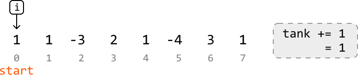
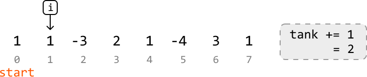



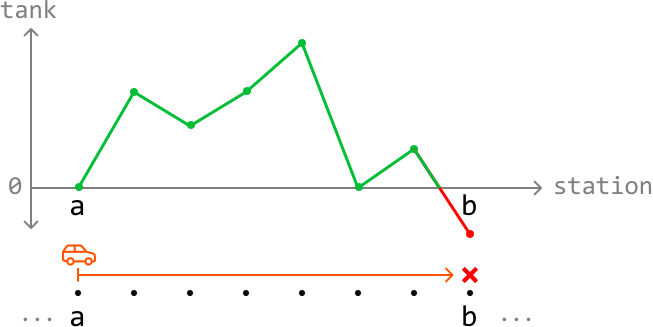
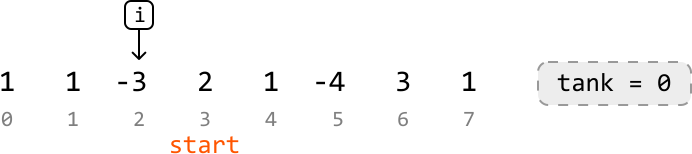
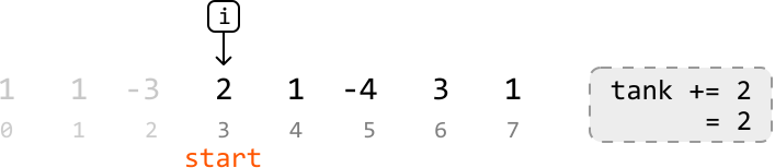
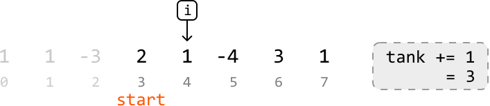

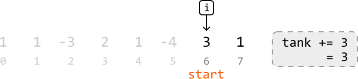
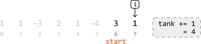


![Image represents two horizontal, one-dimensional arrays of numerical data. The top array, labeled 'ratings = [1 < 3 < 4 < 6 < 8]', contains the numbers 1, 3, 4, 6, and 8, arranged sequentially within square brackets. The numbers are separated by the 'less than' symbol (<), indicating a sorted ascending order. The bottom array, labeled 'candies = [1 2 3 4 5]', displays the numbers 1, 2, 3, 4, and 5, also within square brackets, but without any separating symbols, suggesting a simple sequence. The numbers in the 'candies' array are rendered in orange, while those in the 'ratings' array are in black, except for the '<' symbols which are in a lighter orange. There is no explicit connection or information flow visually depicted between the two arrays; they are presented independently, implying a potential relationship or comparison between the two datasets that is not directly shown in the image itself.](images/img_ee149da9eec0.svg)
![Image represents a diagram illustrating an algorithm or code snippet. At the top, a Python-like list named `ratings` is defined and initialized with the integer values [1, 3, 4, 6, 8]. Below it, another list named `candies` is initialized with [1, 2, 3, 4, 5]. A horizontal arrow connects the second element of `candies` to its last element, indicating an iterative process. Below the arrow, a condition `rating[i] > ratings[i - 1]` is shown, suggesting that the algorithm iterates through the `ratings` list, comparing each element to its preceding element. If the condition is true (the current rating is greater than the previous rating), the subsequent line `candies[i] = candies[i - 1] + 1` indicates that the corresponding element in the `candies` list is incremented by 1. This implies that the number of candies increases only when the rating increases compared to the previous rating. The overall diagram visualizes a conditional update of the `candies` list based on the values in the `ratings` list.](images/img_bbcb4b7e437a.svg)
![Image represents two horizontal arrays of numerical data, presented as Python-style lists. The top array, labeled 'ratings = ', contains the integer sequence [7, 6, 4, 3, 2], with each number separated by a right-pointing arrow symbol ('>'), suggesting a descending order or a comparison between consecutive elements. The bottom array, labeled 'candies = ', displays the integer sequence [5, 4, 3, 2, 1], also in descending order, with the numbers rendered in orange, while the numbers in the 'ratings' array are in black, except for the orange arrows. The two arrays are vertically aligned, implying a potential relationship or correlation between the corresponding elements in each list, possibly illustrating a data structure or a pattern in a coding context.](images/img_1e1b0da2af05.svg)
![The image represents a visual explanation of an algorithm or code snippet that manipulates two arrays, `ratings` and `candies`. The `ratings` array, displayed at the top, contains the integer values [7, 6, 4, 3, 2]. Below it is the `candies` array, initially holding the values [5, 4, 3, 2, 1]. A light-orange horizontal arrow connects the `candies` array, indicating a flow of information or processing from right to left. Below the arrow, the condition `rating[i] > ratings[i + 1]` is shown in orange text, signifying that the algorithm compares consecutive elements in the `ratings` array. If this condition is true (meaning a rating is greater than the next one), the subsequent line, `candies[i] = candies[i + 1] + 1`, in orange text, shows that the corresponding element in the `candies` array is updated by adding 1 to the value of the next element in the `candies` array. This suggests a process where the number of candies assigned is dependent on the relative ranking of ratings, with higher ratings potentially receiving more candies than their lower-rated neighbors.](images/img_51271d8536c4.svg)
![Image represents a line graph illustrating a relationship between 'ratings' and 'candies'. The horizontal axis (x-axis) is labeled 'ratings' and displays a sequence of numbers within square brackets: [4, 3, 2, 4, 5, 1], representing different rating values. The vertical axis (y-axis) is labeled 'candies' and shows a scale from 0 to 3, indicating the quantity of candies. A horizontal line at 'candies = 1' connects six orange data points, each corresponding to a rating value on the x-axis. This visual representation suggests a constant number of candies (one) regardless of the rating value. The graph's structure is simple, with clear axis labels and a straightforward linear relationship between the variables, showing no correlation between the number of candies and the ratings.](images/img_35061aa2d097.svg)
![Image represents a Cartesian coordinate system illustrating a simple data relationship. The horizontal axis, labeled 'ratings,' displays a sequence of numerical ratings: 4, 3, 2, 4, 5, 1, represented along the x-axis with corresponding numerical markers (0, 1, 2, 3, 4, 5) below. The vertical axis, labeled 'candies,' represents a quantity, with values 0, 1, 2, and 3 marked along the y-axis. A horizontal line at y=1 connects six orange dots, each positioned above a rating value on the x-axis. This visually indicates that regardless of the rating (4, 3, 2, 4, 5, or 1), the number of candies remains constant at one. A small black square containing an 'i' is positioned above the data line, with a downward-pointing arrow suggesting it provides additional information or context about the data presented. The x-axis values are enclosed in square brackets, '[ ]', and a right-pointing arrow symbol '>' is placed between the first two rating values (4 and 3).](images/img_7cf646e3d1b2.svg)
![Image represents a line graph illustrating a data set. The horizontal axis is labeled 'ratings' and shows a sequence of numbers from 4 to 1, representing rating values. The vertical axis is labeled 'candies' and shows a scale from 0 to 3, likely representing the quantity or count of candies. A horizontal line at 'candies = 1' connects six data points, each corresponding to a rating value. The data points are represented by orange circles. The x-coordinates of these points are [4, 3, 2, 4, 5, 1] respectively, and their y-coordinate is consistently 1. A small black square containing the letter 'i' is positioned above the data point at rating 2, possibly indicating an information point or annotation related to that specific data point. The x-axis values are presented within square brackets `[ ]`, suggesting a list or array of rating values. A small right-pointing arrow is placed between the rating values 3 and 2, possibly indicating the direction of data flow or sequence.](images/img_ceec017cec6d.svg)
![Image represents a line graph illustrating a relationship between 'ratings' and 'candies'. The horizontal axis displays 'ratings', showing values from 4 to 1, represented as [4, 3, 2, 4, 5, 1] within square brackets. The vertical axis represents 'candies', ranging from 0 to 3. An orange line connects data points, showing the number of candies corresponding to each rating. The line starts at (4,1), remains at a value of 1 for ratings 3 and 2, peaks at (4,2) for the third rating, drops to (5,1) for the fourth rating, and remains at 1 for the final rating of 1. A small black square labeled 'i' is positioned above the peak of the line, with a downward-pointing arrow indicating a possible annotation or additional information related to the highest point on the graph (rating 4, candies 2).](images/img_c2cd03bb9207.svg)
![Image represents a line graph illustrating the relationship between 'ratings' and 'candies'. The horizontal axis (x-axis) is labeled 'ratings' and displays numerical values [4, 3, 2, 4, 5, 1] enclosed in square brackets. The vertical axis (y-axis) is labeled 'candies' and shows values from 0 to 3. An orange line connects data points representing the number of candies corresponding to each rating. The points show that the number of candies starts at 1 for a rating of 4, remains at 1 for ratings of 3 and 2, increases to 2 for a rating of 4, peaks at 3 for a rating of 5, and finally drops to 1 for a rating of 1. A small square box labeled 'i' is positioned above the highest point on the graph, with an arrow pointing downwards to that point, possibly indicating additional information or a key data point.](images/img_38cff0c16329.svg)
![Image represents a line graph illustrating the relationship between 'ratings' (x-axis) and 'candies' (y-axis). The x-axis shows ratings values ranging from 4 to 1, with corresponding numerical indices [0, 1, 2, 3, 4, 5] displayed below. The y-axis represents the number of candies, ranging from 0 to 3. An orange line connects data points, showing the number of candies associated with each rating. The points indicate that at ratings 4 (index 0) and 3 (index 1), there is 1 candy; at rating 2 (index 2), there is also 1 candy; at rating 4 (index 3), there are 2 candies; at rating 5 (index 4), there are 3 candies; and finally, at rating 1 (index 5), there is 1 candy. A small black square with an 'i' inside is positioned to the upper right, with a downward-pointing arrow connecting it to the last data point on the graph, suggesting additional information or context related to that specific data point might be available.](images/img_06947ddfb3c7.svg)
![Image represents a line graph illustrating the relationship between 'ratings' and 'candies'. The horizontal axis (x-axis) represents 'ratings', with values ranging from 0 to 5, shown as [4 3 2 4 5 > 1]. The vertical axis (y-axis) represents 'candies', with values ranging from 0 to 3. An orange line connects data points, showing the number of candies corresponding to each rating. The points are (0,1), (1,1), (2,1), (3,2), (4,3), and (5,1). A small black square labeled 'i' is positioned above the graph, with an arrow pointing downwards towards the data point at (4,3), possibly indicating additional information or a highlight. The graph visually depicts a non-linear relationship, where the number of candies increases initially with ratings, peaks at a rating of 4, and then decreases.](images/img_69a66243de73.svg)
![Image represents a line graph illustrating a relationship between 'ratings' and 'candies'. The horizontal axis (x-axis) displays 'ratings', with values ranging from 4 to 1, represented numerically and with corresponding indices [4<sub>0</sub>, 3<sub>1</sub>, 2<sub>2</sub>, 4<sub>3</sub>, 5<sub>4</sub>, 1<sub>5</sub>] suggesting a possible array or list structure. The vertical axis (y-axis) represents 'candies', with values ranging from 0 to 3. An orange line connects data points, showing the number of candies corresponding to each rating. The points show that the number of candies remains constant at 1 for ratings 4, 3, and 2, then increases to 2 for rating 4, peaks at 3 for rating 5, and finally drops to 1 for rating 1. A small information icon ('i' in a square) points to the data point (4<sub>3</sub>, 2), possibly highlighting a specific data point of interest or an anomaly.](images/img_fd920c0ba6bc.svg)
![Image represents a line graph illustrating a relationship between 'ratings' and 'candies'. The horizontal axis (x-axis) displays 'ratings', with values ranging from 4 to 1, represented numerically and indexed below the axis as [4<sub>0</sub> 3<sub>1</sub> 2<sub>2</sub> < 4<sub>3</sub> 5<sub>4</sub> 1<sub>5</sub>]. The vertical axis (y-axis) represents 'candies', with values from 0 to 3. An orange line connects data points, showing the number of candies corresponding to each rating. The line starts at (4,1), remains at a constant value of 1 until (2,1), then increases sharply to (4,2), peaks at (5,3), and finally drops to (1,1). A small black square labeled 'i' points down to the point (2,1) on the graph, possibly indicating a specific data point of interest or a change in trend.](images/img_7c29b0fbe989.svg)
![Image represents a line graph illustrating the relationship between candy ratings and the number of candies. The horizontal axis, labeled 'ratings,' displays a sequence of ratings represented as a list `[4, 3, 2, 4, 5, 1]`, with each number corresponding to a data point. The vertical axis, labeled 'candies,' represents the quantity of candies, ranging from 0 to 3. An orange line connects data points, showing the number of candies associated with each rating. The points are (4,1), (3,2), (2,1), (4,2), (5,3), and (1,1). A small downward-pointing arrow with an 'i' inside a box is positioned above the point (3,2), possibly indicating additional information or a key data point. The graph visually demonstrates a non-linear relationship between ratings and the number of candies, with the number of candies fluctuating across different rating values.](images/img_602695b3569b.svg)
![Image represents a line graph illustrating a relationship between 'ratings' and 'candies'. The horizontal axis displays 'ratings', with values [4, 3, 2, 4, 5, 1] marked below, each value having a corresponding subscript index [0, 1, 2, 3, 4, 5] indicating the position in the sequence. The vertical axis represents 'candies', ranging from 0 to 3. An orange line connects data points, showing the number of candies corresponding to each rating. The points are (0,3), (1,2), (2,1), (3,2), (4,3), and (5,1). A small square with an 'i' inside is positioned above the first data point (0,3), suggesting additional information might be available. The overall graph depicts a non-linear relationship, where the number of candies fluctuates with changes in ratings.](images/img_a1237d93a508.svg)
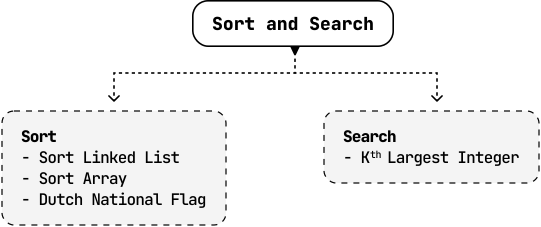
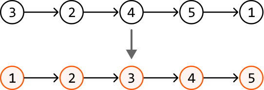
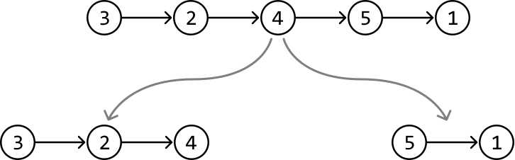

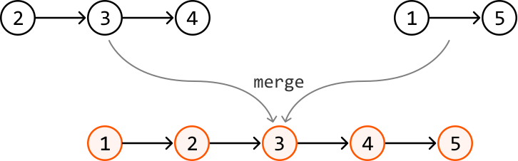
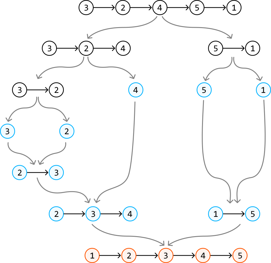
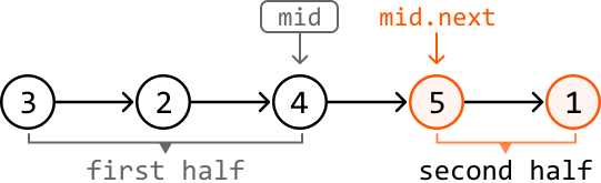





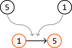
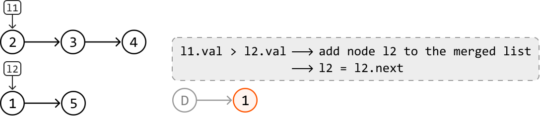
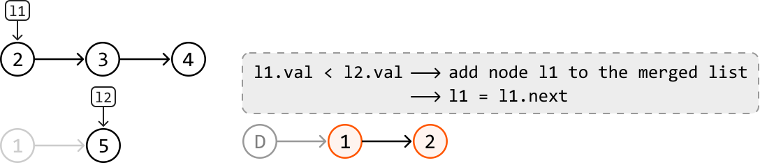
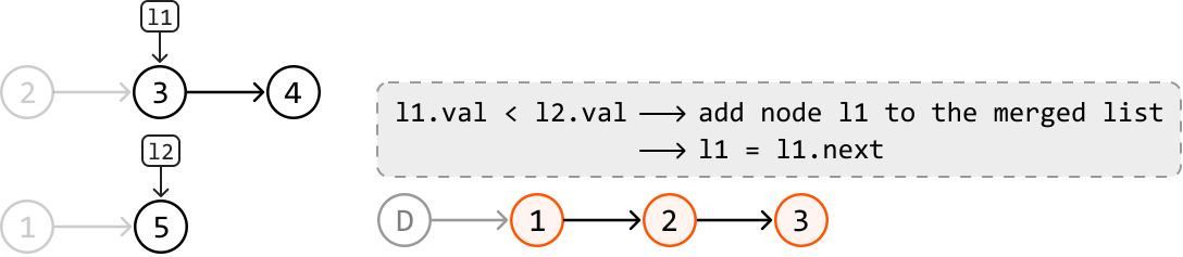
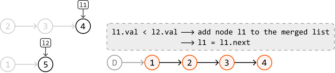
![Image represents a visual depiction of a partitioning step within a sorting algorithm, likely Quicksort. The top row shows an unsorted array [6, 8, 4, 2, 7, 3, 1, 5], with the element '5' highlighted in an orange box and labeled 'pivot'. A downward arrow indicates the partitioning process. The bottom row displays the array after partitioning. The numbers less than the pivot (5) are grouped in a light-blue box labeled 'less than 5' as [4, 2, 3, 1]. The pivot (5) is shown in an orange box, positioned between the two groups, and labeled 'in the correct position'. The numbers greater than the pivot are grouped in a light-purple box labeled 'greater than 5' as [6, 8, 7]. This illustrates how the pivot element is placed in its final sorted position, with all smaller elements to its left and all larger elements to its right, a key step in the Quicksort algorithm.](images/img_b74de16200b0.svg)
![Image represents a sequence of numbers, [6, 8, 4, 2, 7, 3, 1, 5], displayed horizontally. Each number is positioned above its index, indicated in grey text below (0 through 7). The number 5, located at index 7, is highlighted within an orange rectangular box, labeled 'pivot' in orange text to its upper right. The arrangement visually depicts a data array, with the highlighted '5' signifying a pivot element within the context of a sorting algorithm or similar data structure operation. No URLs or parameters are present; the image solely illustrates the positional relationship between the numbers and the designated pivot.](images/img_00e04718a0c2.svg)
![Image represents a visual depiction of a portion of a sorting algorithm, likely Quicksort. The diagram shows an array `[6, 8, 4, 2, 7, 3, 1, 5]` with indices 0 through 7 displayed below each element. Above the array, two boxes labeled '10' (light gray) and 'i' (black) indicate variables. Arrows point from both '10' and 'i' downwards, suggesting these variables are used to iterate through the array. To the right, a separate box labeled 'pivot' contains the value '5', indicating the pivot element for this iteration. A dashed-line box depicts a conditional statement: 'nums[i] > pivot'. An arrow extends from this condition to the word 'continue,' illustrating that if the condition `nums[i] > pivot` is true, the algorithm continues to the next iteration. The overall diagram illustrates a single step in the partitioning phase of a sorting algorithm, where elements are compared to the pivot to determine their position in the sorted array.](images/img_e63e3aeb86ff.svg)
![Image represents a snapshot of a sorting algorithm, likely Quicksort, illustrating a single iteration. A numerical array `[6, 8, 4, 2, 7, 3, 1, 5]` is shown with indices 0 through 7 displayed below each element. A grey box labeled 'lo' (likely representing the lower index of a partition) points to the element '6' at index 0, and a black box labeled 'i' (likely representing the current index) points to the element '8' at index 1. A dashed arrow connects 'lo' to 'i', suggesting a comparison or traversal between these indices. A separate grey box labeled 'pivot' contains the value '5', indicating the pivot element selected for this partition. A decision box with dashed borders shows a condition: `nums[i] > pivot`. If this condition is true (as it is for '8'), a solid arrow points to the word 'continue', implying the algorithm proceeds to the next iteration, potentially incrementing 'i' to compare the next element. The overall diagram visualizes the state of the algorithm during a comparison step within the partitioning phase of a sorting algorithm.](images/img_84dae8ec1fbf.svg)
![Image represents a visual depiction of a step in a sorting algorithm, likely Quicksort. A numerical array `[6, 8, 4, 2, 7, 3, 1]` is shown, with indices 0 through 6 displayed below each element. Above the array, two boxes labeled '10' (grey) and 'i' (black) indicate variables. A downward arrow from '10' points to the element '6' at index 0, suggesting '10' might represent the array's length or a related parameter. A downward arrow from 'i' points to the element '4' at index 2. A dashed curved arrow connects 'i' to '8' at index 1, indicating a comparison or swap operation. Finally, a separate box labeled 'pivot' contains the value '5', suggesting '5' is the pivot element selected for this partitioning step in the algorithm. The arrangement visually demonstrates the algorithm's progress in partitioning the array around the pivot.](images/img_667bd019bf1c.svg)
![Image represents a visual depiction of a step within a sorting algorithm, likely Quicksort. The left side shows an array `[6, 8, 4, 2, 7, 3, 1, 5]` with indices 0 through 7 displayed below each element. Arrows point downwards from labeled boxes 'lo' (initially pointing to index 0) and 'i' (initially pointing to index 2) indicating their current positions within the array. The number 5 is labeled as 'pivot'. The right side shows a decision box with dashed borders. This box contains a condition `nums[i] < pivot`, which checks if the element at index `i` (currently 4) is less than the pivot (5). If true, two actions are performed: `swap(nums[i], nums[lo])` swaps the element at index `i` with the element at index `lo`, and `lo += 1` increments the `lo` index. The arrows from the decision box represent the flow of control based on the condition's outcome. The overall diagram illustrates a single iteration of the partitioning phase in a sorting algorithm, where elements smaller than the pivot are moved to the left side of the array.](images/img_8936b1b4fb40.svg)
![Image represents a step in a sorting algorithm, likely Quicksort, illustrating a swap operation. The array `[4, 8, 6, 2, 7, 3, 1]` is shown with indices 0 through 6 displayed below each element in gray. A light-blue box labeled 'lo' points down to the element at index 0 (value 4), and a black box labeled 'i' points down to the element at index 2 (value 6). A curved light-blue arrow labeled 'swapped' connects the element at index 0 (4) to the element at index 2 (6), indicating these two elements have been exchanged. To the right, a gray box labeled 'pivot' contains the value 5, which is likely the pivot element around which the partition is being built. The arrangement visually depicts the state of the array during the partitioning phase of the algorithm, where elements smaller than the pivot are moved to the left and larger elements to the right.](images/img_a1b13cc610ac.svg)
![Image represents a visual depiction of a step in a sorting algorithm, likely Quicksort. An array [4, 8, 6, 2, 7, 3, 1] is shown with indices 0 through 6 displayed below each element. A light-blue box labeled 'lo' (likely representing the low index) points to the element '8' at index 1 via a dashed arrow indicating a potential swap or comparison. A black box labeled 'i' (likely representing the iterator or current index) points to the element '6' at index 2 with a solid arrow. A grey box labeled 'pivot' contains the value '5' at index 7, indicating this element is the pivot around which the partition is being formed. The arrangement shows the algorithm's progress in partitioning the array based on the pivot value. The dashed arrow from 'lo' suggests a comparison or movement of the '8' element relative to the pivot. The solid arrow from 'i' indicates the iterator's position in the array during the partitioning process.](images/img_5cddfc590753.svg)
![The image represents a visual depiction of a pivot element in an array during a sorting algorithm, likely Quicksort. A numerical array `[4, 2, 3, 1, 8, 6, 7, 5]` is shown, with indices 0 through 7 displayed below each element. Elements 4, 2, and 3 are colored light blue, indicating they might be processed or sorted already. The number 1 is also light blue, suggesting it's part of a sorted or processed section. The number 8, 6, and 7 are in black, implying they are yet to be processed. A light gray box labeled 'pivot' contains the number 5, located at index 7, signifying it's the chosen pivot element for this iteration. A light blue box above the array contains the number '10,' which might represent the total number of elements or a related parameter. A downward-pointing arrow connects the '10' box to the number 8 in the array, possibly indicating the pivot selection process or the current position of the algorithm's pointer.](images/img_6a8a92b474b4.svg)
![Image represents a visual depiction of a single step in a sorting algorithm, likely Quicksort. The image shows an array [4, 2, 3, 1, 5, 6, 7, 8] with indices 0 through 7 displayed below each element. The number 5 is highlighted in a light beige box with an orange border and labeled 'pivot'. A curved orange arrow connects the element 1 (at index 3) and the element 8 (at index 7), labeled 'swapped,' indicating that these two elements have been exchanged during the partitioning phase of the algorithm. The arrangement visually demonstrates the in-place swapping of elements relative to the pivot element during the partitioning process of a sorting algorithm.](images/img_ca831523dcb9.svg)
![Image represents a simple array or list data structure depicted using square brackets `[]` to enclose five integer elements: 1, 2, 3, 4, and 5. These elements are arranged sequentially within the brackets, separated by spaces, indicating their order within the data structure. No connections or information flow is explicitly shown beyond the inherent sequential arrangement of the elements within the array. The image solely illustrates the basic structure of a list containing five integers, with no further metadata, labels, or external connections depicted.](images/img_f18236d34e8e.svg)
![Image represents a visual depiction of a partitioning step within a sorting algorithm, likely Quicksort. The illustration shows an array represented as `[1 2 3 4 5]`. The number 5 is highlighted in an orange box and labeled 'pivot'. A light-blue rounded rectangle encloses the numbers 1, 2, 3, and 4, labeled 'left part' in light-blue text. A purple arrow originates from the right side of the pivot (5) and points to the right, indicating the absence of a 'right part' in this specific step. The overall arrangement demonstrates the partitioning process where elements smaller than the pivot are placed to its left, and in this case, no elements are larger than the pivot, resulting in an empty right partition.](images/img_608ba06de0d2.svg)
![Image represents a visual depiction of a partitioning step in a sorting algorithm, likely Quicksort. The image shows a numerical array `[1, 2, 3, 4]` enclosed in square brackets. The first three elements, `[1, 2, 3]`, are grouped together in a light-blue rounded rectangle and labeled in light-blue text as 'left part'. The last element, `4`, is separately enclosed in an orange rounded rectangle and labeled above in orange text as 'pivot'. A purple arrow originates from the bottom of the 'pivot' rectangle and points to the right, indicating the direction of data flow, and is labeled in purple text as 'no right part'. This illustrates a scenario where the pivot element is already in its correct sorted position, resulting in an empty right partition after the partitioning step. The arrangement visually separates the array into a 'left part' and an implicitly empty 'right part' based on the pivot's position.](images/img_c062cd610b84.svg)
![Image represents a visual explanation of a counting sort algorithm. At the top, a list named `nums` is shown, containing the integer values [2, 1, 0, 0, 2, 4, 2]. A gray line underlines this list. Below, a list called `counts` is displayed, representing the frequency of each element in `nums`. `counts` contains [2, 1, 3, 0, 1], indicating two 0s, one 1, three 2s, zero 3s, and one 4. Small gray numbers (0, 1, 2, 3, 4) are placed above `counts` to clarify the index corresponding to each element's count. Orange curved arrows connect each element in `counts` to the corresponding number of elements in the final `res` list. `res` is the sorted output list, shown at the bottom as [0, 0, 1, 2, 2, 2, 4], where each element's position reflects its sorted order based on the counts in the `counts` list. The arrows visually demonstrate how the frequency information in `counts` is used to populate the sorted `res` list.](images/img_47bed20c6c98.svg)
![Image represents a visual explanation of finding the k<sup>th</sup> largest element in an array. The diagram begins with an unsorted array `[5 2 4 3 1 6]` where `k` is defined as 3. The array's elements are indexed from 0 to 5, shown below each element. A rightward arrow labeled 'sort' indicates a sorting operation transforming the initial array into a sorted array `[6 5 4 3 2 1]`, maintaining the same indexing. Above the sorted array, an orange arrow points down to the element at index 2 (the third largest element), which is 4, highlighting that the 3<sup>rd</sup> largest element (k=3) is 4. The element '4' is circled in a peach color to emphasize its selection as the k<sup>th</sup> largest element.](images/img_fc91b36bfe6b.svg)
![Image represents a visual depiction of finding the top k largest elements from a list. The input is shown as a list `[5 2 4 3 1 6]` enclosed in square brackets, with each number circled in orange. Arrows in orange indicate the selection of the three largest numbers (5, 4, and 6). These three numbers are then collected into a new list `[5 4 6]`, labeled 'top k largest:', with the number 4 highlighted in a light green circle. A green downward-pointing arrow from the light green circle points to the word 'min', suggesting a subsequent step might involve finding the minimum element within the top k largest elements. The overall diagram illustrates a process of selecting the top k elements and potentially further processing them.](images/img_8bfd1b890298.svg)
![Image represents a visual depiction of a min-heap data structure being populated. A downward-pointing arrow originates from a small square containing the letter 'i', suggesting an input source. This arrow points to a bracketed array `[5 2 4 3 1 6]`, where each number represents an element, and the subscripts (0, 1, 2, 3, 4, 5) indicate their indices within the array. To the right, a trapezoidal shape labeled 'min_heap' visually represents the min-heap structure. The number '5' is shown at the top of the min-heap, indicating that it's the root node (the smallest element). The image illustrates the initial step of building a min-heap, where the first element from the input array (5) is placed at the root of the min-heap. The remaining elements (2, 4, 3, 1, 6) are implicitly implied to be added subsequently to maintain the min-heap property (where the value of each node is less than or equal to the values of its children).](images/img_a5f01eac13c7.svg)
![Image represents a visual depiction of a min-heap data structure being built. A downward-pointing arrow labeled 'i' points to an array `[5, 2, 4, 3, 1, 6]`, where each element's index (0-5) is shown below it in gray. This array represents the input data. To the right, a min-heap is shown, visually represented as a trapezoidal structure with a purple border and labeled 'min_heap'. The top node contains the value '2', and the bottom node contains the value '5'. The diagram illustrates an intermediate step in the process of constructing a min-heap from the input array; the '2' at the top of the min-heap suggests that the algorithm has already processed at least the first few elements of the array, placing the smallest element found so far at the root of the heap. The remaining elements in the array are yet to be incorporated into the min-heap structure.](images/img_8d14c733a5fc.svg)
![Image represents a visual depiction of a data structure transformation. A small square labeled 'i' points downwards to an array `[5, 2, 4, 3, 1, 6]`, where each element is indexed from 0 to 5 below it. This array is being transformed into a min-heap data structure, shown as a trapezoidal shape with a purple outline labeled 'min_heap'. The min-heap contains the numbers 2, 4, and 5, arranged such that 2 is at the top, 4 is below and to the left, and 5 is below and to the right. The arrangement suggests that the value of each node is less than or equal to the values of its children, a defining characteristic of a min-heap. The arrow from 'i' implies that the array is the input to the process of creating the min-heap.](images/img_ea65117c165a.svg)
![Image represents a step-by-step illustration of a coding pattern involving a min-heap data structure. The top left shows an array `nums` with elements [5, 2, 4, 3, 1, 6], indexed from 0 to 5, with an arrow pointing to the element at index 3 (value 3). To the right, a min-heap is depicted, initially containing elements 4 and 5, with a 2 (crossed out in red) at the top, indicating it's about to be removed. A dashed box next to the heap describes the algorithm: if `nums[i]` (the current element being processed from the array) is greater than the top element of the min-heap, then the top element is popped (in this case, 2), and `nums[i]` (which is 3) is pushed onto the min-heap. The bottom part shows the min-heap after this operation, now containing 3, 4, and 5. The arrow connecting the top and bottom min-heap diagrams visually represents the transformation resulting from the algorithm described in the dashed box.](images/img_82fa1f2b0213.svg)
![Image represents a step in an algorithm, likely involving a min-heap data structure. A numbered array `[5 2 4 3 1 6]` is shown, with an index `i` (represented by a box labeled 'i') pointing to the element '1' at index 4. A min-heap is depicted visually as a tree structure with elements 3 (at the top), 4, and 5. The label 'min_heap' is below the heap. A downward arrow from 'i' points to the array element '1', indicating the current element being processed. A dashed box contains the condition `nums[i] < min_heap.top`, which checks if the current array element (1) is less than the top element of the min-heap (3). A right-pointing arrow from this condition indicates that if the condition is true, the algorithm continues. The overall diagram illustrates a comparison between an element from an input array and the top element of a min-heap, a common operation in heap-based algorithms like heapsort or priority queue management.](images/img_68cd727541d8.svg)
![Image represents a step-by-step illustration of a coding pattern involving a min-heap data structure. The top section shows an array `nums` with elements [5, 2, 4, 3, 1, 6] indexed from 0 to 5, and a min-heap represented as a purple triangle containing the values 4 and 5. A downward arrow points from an index `i` (represented by a small square labeled 'i') to the min-heap, indicating that the element at index `i` (which is 1 in this case) is being processed. A separate box describes the condition `nums[i] > min_heap.top` and the actions taken if the condition is true: popping the top element (3) from the min-heap and pushing `nums[i]` (1) onto the min-heap. The bottom section shows the resulting min-heap after these operations, now containing 4, 5, and 6, illustrating the updated state of the min-heap after processing the element at index `i`. A horizontal arrow connects the before and after states of the min-heap.](images/img_dc04afcb2ce4.svg)
![Image represents a comparison of three different approaches to sorting an array. The input array `[5 2 4 3 1 6]` is shown at the left. Three arrows emanate from this array, each representing a different sorting method. The top arrow leads to a fully sorted array `[1 2 3 4 5 6]`, labeled 'sort the whole array:', with a time complexity of O(nlog(n)). The middle arrow points to a partially sorted array `[... 4 5 6]`, labeled 'sort the k largest integers:', showing only the k largest integers sorted, with a time complexity of O(nlog(k)). The bottom arrow shows a final array `[... 4 ...]`, labeled 'only position the k<sup>th</sup> largest integer in its sorted index:', where only the k<sup>th</sup> largest integer (in this case, 4) is placed in its correct sorted position. This last method is marked with '(faster?)', suggesting it's potentially more efficient than the previous two. Each array displays indices below its elements for clarity. The highlighted '4' in each output array emphasizes the focus on the k<sup>th</sup> largest element.](images/img_82c3df55783d.svg)
![Image represents a visual explanation of finding the kth largest element in an array using the `quickselect` algorithm. The diagram shows an initial unsorted array `[5 2 4 3 1 6]` with indices 0 through 5 displayed below each element. Above the array, the equation 'k<sup>th</sup> largest == (n - k)<sup>th</sup> smallest' highlights the relationship between the kth largest and (n-k)th smallest elements, where 'n' is the array's size. A horizontal arrow connects the initial array to a partially sorted array `[2 1 3 4 5 6]`. This arrow is labeled `quickselect(n - k)`, indicating that the `quickselect` function is applied to find the (n-k)th smallest element. The (n-k)th smallest element (which is also the kth largest) is highlighted in light green within the resulting array, specifically at index `n - k`, which is explicitly labeled with a green upward-pointing arrow. The diagram visually demonstrates how finding the (n-k)th smallest element using `quickselect` effectively identifies the kth largest element.](images/img_e369f18a7d12.svg)
![Image represents a segment of a Quickselect algorithm visualization. At the top, a conditional statement 'if pivot_index < n - k:' is shown, indicating a decision point in the algorithm. Below this, a visual representation of an array is presented. The array is shown as `[ . . pivot . . . . ]`, where `pivot` is a gray square representing the pivot element, and the dots represent other elements. A peach-colored rectangle highlights a portion of the array to the right of the pivot. A green upward-pointing arrow labeled 'index n - k' connects to the right side of this peach rectangle, indicating that this section of the array contains `n - k` elements, where `n` is the array's size and `k` is a target rank. Finally, a light gray, dashed-bordered box to the right states 'perform quickselect on the right part,' indicating that if the condition `pivot_index < n - k` is true, the Quickselect algorithm recursively operates on the right sub-array (the peach-colored section) to find the k-th smallest element.](images/img_0954e3b79b00.svg)
![Image represents a segment of a Quickselect algorithm flowchart. The top shows a conditional statement: `if pivot_index > n - k:`. Below this, a peach-colored rectangle represents an array, depicted with ellipses (...) indicating multiple elements, enclosed in square brackets `[ ... ]`. A single element within the array is highlighted as `pivot` within a grey square. A green upward-pointing arrow labeled `index n - k` connects the array to the `pivot` element, indicating its position within the array. To the right, a dashed-line rectangle contains the text 'perform quickselect on the left part', describing the action taken if the conditional statement is true. The overall structure illustrates a decision point in the algorithm: if the pivot's index is greater than `n - k`, then the Quickselect algorithm is recursively applied to the left portion of the array.](images/img_a83f99cfc404.svg)
![Image represents a code snippet illustrating a conditional return statement within a function. The top line shows a conditional statement: `if pivot_index == n - k:`. This checks if the variable `pivot_index` is equal to the result of `n - k`, where 'n' and 'k' are presumably pre-defined variables. Below this, a visual representation of an array `[...]` is shown, with ellipses (...) indicating unspecified elements. A light-green square labeled 'pivot' highlights a specific element within the array. An upward arrow points from the text 'index n - k' to the 'pivot' square, indicating that `pivot_index` represents the index `n - k` within the array `nums`. To the right, a dashed-line box contains the code `return nums[pivot_index]`, signifying that if the condition in the first line is true, the function returns the element at the `pivot_index` within the `nums` array. The overall diagram visually explains how a pivot element's index is calculated and used to return a value from an array based on a specific condition.](images/img_a2fb98ef972a.svg)
![Image represents a visual explanation of a sorting algorithm, specifically illustrating how elements naturally group during the process. The diagram shows an unsorted array `[2 0 1 2 0 0 1]` where numbers 0 are colored red, 1s are black, and 2s are cyan. A thick black arrow points to a sorted array `[0 0 0 1 1 2 2]`. Underneath the sorted array, red and cyan horizontal brackets highlight the groups of 0s and 2s respectively, labeled 'sort 0s' and 'sort 2s' in their respective colors. Above the sorted array, a black bracket highlights the group of 1s, with the text '1s will naturally get sorted' explaining their position. The overall arrangement demonstrates how, without explicit sorting of 1s, the algorithm implicitly places them in their correct sorted position between the 0s and 2s.](images/img_b4dc2dfe2ed5.svg)
![Image represents a one-dimensional array or list depicted using square brackets `[]`. The array contains seven integer elements: 2, 0, 1, 2, 0, 0, and 1. These elements are displayed in bold, black font and are arranged sequentially within the brackets. Below the array, a sequence of numbers from 0 to 6 is shown in a lighter gray font; these numbers represent the indices of the corresponding elements in the array, starting from index 0 for the first element (2) and ending at index 6 for the last element (1). There is no explicit information flow or connections between the elements other than their sequential arrangement within the array structure indicated by the brackets and the implicit index mapping provided by the numbers below.](images/img_4ea9acd83c16.svg)
![Image represents a visual depiction of a sorting algorithm's step, likely part of a quicksort or similar algorithm. Two labeled boxes, 'left' and 'i' (likely representing an index), point downward with arrows to an array `[2 0 1 2 0 0 1]`, indicating that the algorithm is focusing on the element at index `i` (which is 2 in this case). A separate box labeled 'right' points to the last element of the array (1). A dashed-bordered box to the right details the algorithm's logic: `nums[i] == 2` shows the value at index `i`; `→ swap(nums[i], nums[right])` indicates that the algorithm will swap the element at index `i` (value 2) with the element at the 'right' index (value 1); and `→ right--` shows that the 'right' index will be decremented after the swap. The numbered indices beneath the array clarify the positions of each element within the array. The overall diagram illustrates a single iteration of a sorting algorithm's partitioning step, focusing on the comparison and potential swap of elements based on their values relative to a pivot (implicitly defined by the 'right' index).](images/img_9966fefcfe24.svg)
![Image represents a visual depiction of a sorting algorithm, likely a variation of quicksort or similar, showing a single swap operation. A numerical array `[1 0 1 2 0 0 2]` is displayed, with indices 0 through 6 shown below each element. Two rectangular boxes labeled 'left' (in gray) and 'right' (in light blue) point downwards with arrows to the array's first and last elements, respectively. A smaller gray box labeled 'i' is positioned near the 'left' box, suggesting an index or pointer. A curved, light-blue arrow labeled 'swapped' connects the first and last elements (1 and 2), indicating that these elements have been exchanged during the sorting process. The arrows from 'left' and 'right' highlight the elements selected for comparison and subsequent swapping.](images/img_e2f949b1a6c8.svg)
![Image represents a visual depiction of a two-pointer approach to array manipulation. Two labeled boxes, 'left' (gray) and 'right' (light blue), point downwards towards an array `[1 0 1 2 0 0 2]`. The array's indices are displayed below it, ranging from 0 to 6. The 'left' pointer initially targets the first element (index 0), while the 'right' pointer points to the last element (index 6). A small, dark gray box labeled 'i' is positioned next to the 'left' box, suggesting an index variable. A dashed, light blue arrow from the 'right' pointer indicates that it might move leftward during the algorithm's execution. The downward arrows from 'left' and 'right' visually represent the pointers' initial positions within the array. The overall diagram illustrates the starting configuration of a common algorithm that likely involves processing the array from both ends, possibly for sorting, searching, or other operations requiring bidirectional traversal.](images/img_014f41c35085.svg)
![Image represents a visual depiction of a code snippet likely involving array traversal and conditional logic. The diagram shows a numerical array `[1 0 1 2 0 0 2]` with indices displayed below each element (0 through 6). A rectangular box labeled 'left' points to the array's first element (at index 0), and another box labeled 'i' (likely representing an index variable) points to the same element. A downward-pointing arrow from 'i' indicates that the variable `i` is currently pointing to the first element of the array. A separate box labeled 'right' points to the array's element at index 5. A dashed-line box to the right describes a conditional statement: `nums[i] == 1`, which checks if the element at the index `i` is equal to 1. If this condition is true, an action `i++` (incrementing the index `i`) is performed, implying that the code iterates through the array, checking each element for the value 1 and moving to the next element if found.](images/img_aa5ca4997eca.svg)
![Image represents a visual depiction of a two-pointer approach to array traversal. A numerical array `[1, 0, 1, 2, 0, 0, 2]` is shown, with each element's index displayed below it (0 through 6). Two rectangular boxes labeled 'left' and 'right' point downwards, indicating pointers to the array's beginning and end, respectively. A square box labeled 'i' points downwards to the second element (value 0) of the array. A dashed arrow connects the 'left' pointer (pointing to the first element, value 1) to the 'i' pointer, suggesting an interaction or comparison between these two elements. The 'right' pointer points to the second-to-last element (value 0). The arrangement visually demonstrates the concept of using two pointers, 'left' and 'right,' to traverse and potentially manipulate an array, with the 'i' pointer possibly representing an intermediate index or a point of comparison within the array. The grayscale variation in the array's element indices suggests a possible focus on a specific sub-section of the array during the traversal.](images/img_74abcca04323.svg)
![Image represents a visual depiction of a step within a sorting algorithm, likely a variation of quicksort. The top shows two labeled boxes, 'left' (in red) and 'i' (in black), pointing down with arrows to the array `[1 0 1 2 0 0 2]`. The 'left' arrow points to the element '1' at index 0, and the 'i' arrow points to the element '0' at index 1. A third box labeled 'right' (in grey) points to the element '0' at index 4. A dashed-line box to the right contains a conditional statement 'nums[i] == 0' followed by an action '→ swap(nums[i], nums[left])'. This indicates that if the element at index `i` (which is 0) is equal to 0, then the algorithm swaps the values at indices `i` and `left`. The indices are shown below the array elements for reference. The diagram illustrates a single iteration where the algorithm checks a specific element and performs a swap based on a condition.](images/img_9ca400996499.svg)
![Image represents a visual depiction of a sorting algorithm, likely a variation of quicksort or similar, showing a single swap operation. A red box labeled 'left' points down to the first element (0) of an array [0, 1, 1, 2, 0, 0, 2]. A gray box labeled 'i' points down to the second element (1) of the same array. Below the array, index numbers (0, 1, 2, 3, 4, 5, 6) are shown for reference. A red curved arrow labeled 'swapped' indicates that the elements at indices 0 and 1 have been exchanged. A gray box labeled 'right' points down to the array's element at index 4 (the first 0 after the initial elements). The visual emphasizes the interaction between the 'left' and 'i' pointers during a single swap step within a larger sorting process, highlighting the movement and exchange of elements based on their values and the pointers' positions.](images/img_32d188e70346.svg)
![Image represents a visual depiction of a coding pattern, likely illustrating array manipulation. The diagram shows a numerical array `[0 1 1 2 0 0 2]` with indices displayed below (0 to 6). Above the array, two labeled boxes, 'left' (in red) and 'i' (in gray), point downwards with arrows to the array's elements at indices 0 and 1 respectively. Another labeled box, 'right' (in gray), points to the element at index 5. To the right, a dashed-line box indicates the resulting actions: two arrows point to 'left++' and 'i++', suggesting that the variables 'left' and 'i' are incremented after accessing their respective array elements. The overall pattern suggests an iterative process involving two pointers ('left' and 'i') moving through the array, potentially for comparison or manipulation, with the 'right' pointer possibly indicating a boundary or target.](images/img_fccaab655da0.svg)
![Image represents a visual depiction of a data structure manipulation, possibly within an algorithm. A numerical array `[0, 1, 1, 2, 0, 0, 2]` is shown, with each element indexed below (0-6). Two labeled boxes, 'left' (red) and 'right' (gray), indicate operations on the array. A solid black arrow descends from 'left' to the element '1' at index 1, signifying a direct modification or access. A solid black arrow descends from 'i' (a gray box likely representing an index or iterator) to the element '1' at index 2, indicating another direct modification or access. A dashed red arrow connects 'left' to the element '0' at index 0, suggesting a potential indirect influence or conditional operation. A solid gray arrow descends from 'right' to the element '0' at index 5, showing a direct modification or access at that location. The overall image illustrates how different parts of an array are accessed and potentially modified from different points of reference ('left' and 'right'), possibly within a sorting or merging algorithm.](images/img_39ed1022dd1f.svg)
![Image represents a diagram illustrating a coding pattern, possibly related to array traversal or searching. Three rectangular boxes labeled 'left,' 'right,' and 'i' are positioned above a numerical array represented as `[0 0 0 1 1 2 2]`, with indices 0 through 6 displayed below the array elements. Arrows descend from 'left,' 'right,' and 'i' pointing to specific elements within the array: 'left' points to '1' at index 3, 'right' points to '1' at index 4, and 'i' points to '2' at index 5. The array elements at indices 0, 1, and 2 are colored red, suggesting they might be excluded or processed differently. The element at index 4 is colored light blue, suggesting a different state. A separate, dashed-line box to the right displays the condition 'i > right → stop,' indicating that the algorithm terminates when the value of 'i' exceeds the value of 'right'. The overall diagram depicts a process where two pointers ('left' and 'right') and an index ('i') traverse an array, potentially searching or manipulating its elements based on the condition specified in the final box.](images/img_34ad55b623b7.svg)
![The image represents a visual depiction of a merge operation, likely within a merge sort algorithm. Two labeled sources, 'left' (in red) and 'right' (in gray), each point downwards via arrows to an array-like structure. The 'left' source points to the first element, '0', of the array [0, 1, 2], with the index '0' shown below it. The 'i' box, in black and white, also points to the same array's first element, suggesting an index or iterator. The 'right' source points to the element '1' in the array [1], with the index '3' shown below it. The arrays are presented side-by-side, implying that the merge operation combines elements from two sorted sub-arrays ('left' and 'right') into a single sorted array. The arrows visually represent the flow of data from the source arrays into the merged array, illustrating the merging process.](images/img_6d89937ba13e.svg)
![Image represents a visual depiction of a step in a sorting algorithm, likely a partitioning step within quicksort. The left side shows an array `[0, 1, 2, 1]` with indices 0, 1, 2, and 3 displayed below. A red box labeled 'left' points to the element at index 0 (value 0), and a gray box labeled 'i' points to the element at index 1 (value 1). A red arrow indicates a connection from 'left' to the element at index 0, suggesting a pointer or index variable. A black arrow from 'i' also points to the element at index 1. A gray box labeled 'right' points to the element at index 3 (value 1). The right side shows a pseudocode block describing the algorithm's logic. It checks if `nums[i]` (the element pointed to by 'i') is equal to 0. If true, it executes `swap(nums[i], nums[left])`, swapping the elements at indices `i` and `left`. Finally, it increments `left` using `left++`, moving the 'left' pointer one position to the right. The overall diagram illustrates the process of partitioning an array based on a pivot value (likely 0 in this case) by comparing elements and swapping them to place elements smaller than the pivot to the left.](images/img_d838eac5bae7.svg)
![Image represents a visual depiction of an iterative process, likely within a loop in a program. A gray box labeled 'i' represents a loop counter variable. A red box labeled 'left' and a gray box labeled 'right' represent index pointers or variables. Arrows indicate the flow of control. A downward arrow from 'i' points to the element at index 0 in the array `[0, 1, 2, 1]`. A downward red arrow from 'left' points to the element at index 1. A dashed red arrow connects the element at index 0 to the element at index 1, suggesting a comparison or operation between these elements. A downward gray arrow from 'right' points to the element at index 3. The array `[0, 1, 2, 1]` is indexed from 0 to 3, shown below the array. The condition `(i < left)` is displayed, indicating a loop continuation condition where the loop continues as long as the value of `i` is less than the value of `left`. The overall diagram illustrates a step in an algorithm, possibly a search or sorting algorithm, that involves comparing and manipulating elements within an array using index pointers.](images/img_072d2a95790b.svg)
![Image represents a visual depiction of a step in a sorting algorithm, likely a variation of quicksort or similar. The left side shows an array `[0, 1, 2, 1]` with indices 0, 1, 2, and 3 displayed below. A red box labeled 'left' points to the element at index 0 (value 0), and a gray box labeled 'i' points to the element at index 0 (value 0) as well. A gray box labeled 'right' points to the element at index 3 (value 1). The right side shows a pseudocode block describing the algorithm's actions. The first line checks if `nums[i]` (the element at index `i`) is equal to 0. If true, the next line executes `swap(nums[i], nums[left])`, swapping the element at index `i` with the element at index `left`. The following lines increment `left` (`left++`) and `i` (`i++`), moving to the next elements in the array. The arrows visually connect the code block to the array, illustrating the flow of data and control during the algorithm's execution. The red arrow from 'left' to the array element 0 highlights the current position of the 'left' pointer.](images/img_181ff4a95251.svg)
![Image represents a visual depiction of an array manipulation process, likely within a sorting or searching algorithm. A numerical array `[0, 1, 2, 1]` is shown, with indices 0, 1, 2, and 3 displayed below each element. A red box labeled 'left' points with a solid red arrow to the element '1' at index 1, indicating a selection or operation on this element. A dashed red arrow from 'left' curves to the element '0' at index 0, suggesting a comparison or potential swap. A gray box labeled 'i' points with a solid black arrow to the same element '1' at index 1, possibly representing an iterator or index variable. Finally, a gray box labeled 'right' points with a solid gray arrow to the element '1' at index 3, potentially indicating another element involved in the comparison or operation. The overall diagram illustrates the interaction between different parts of an algorithm, focusing on the element at index 1 and its relationship to other elements within the array, possibly during a left-to-right traversal or comparison.](images/img_f393d58c0f95.svg)

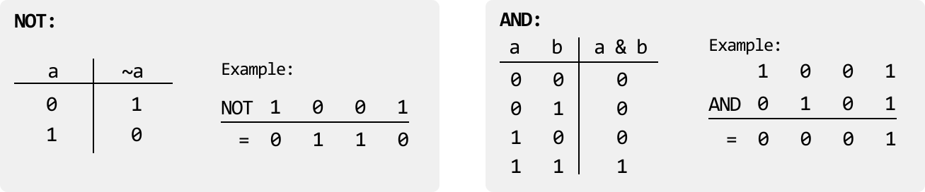
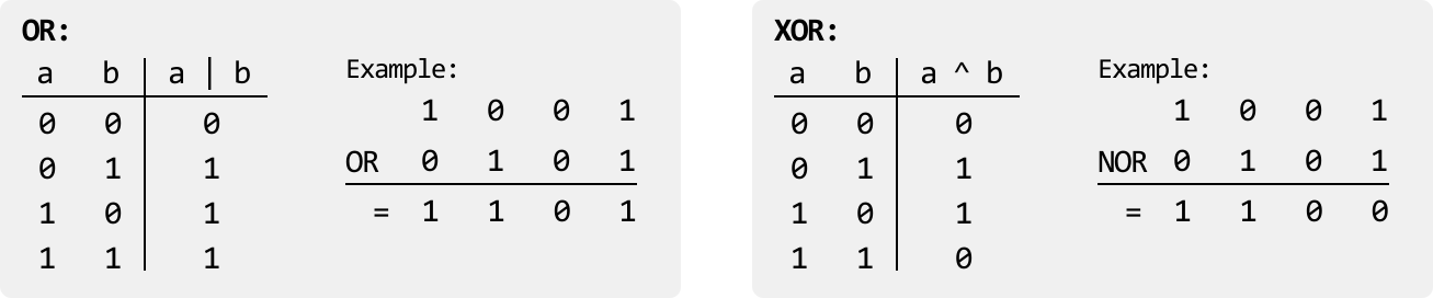
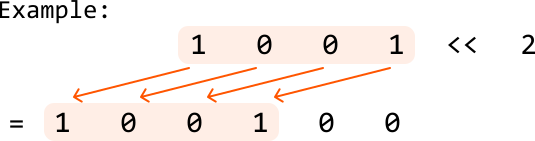
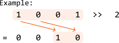
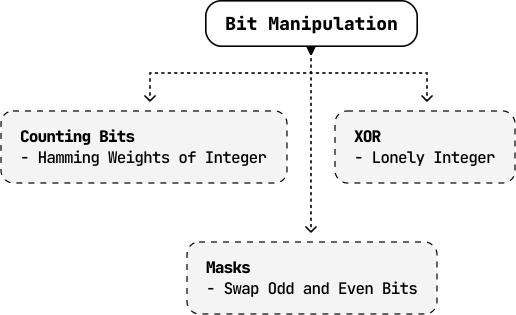

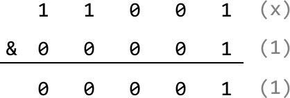
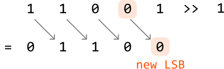
![Image represents a diagram illustrating a bitwise right shift operation. The top row shows an initial value `x` represented by two encircled '1's, followed by three '0's. A blue arrow labeled 'LSB' points downwards, indicating the least significant bit is being processed. Grey arrows connect each bit in the top row to the corresponding bit in the bottom row. The top row represents the initial value of `x`, and the bottom row shows the result of the right shift operation (`x >> 1`). The encircled '1's in the top row shift one position to the right, resulting in the encircled '1's in the bottom row. The remaining bits are filled with '0's. To the right, `dp[x] = 2` indicates the initial count of '1's in `x`, and `dp[x >> 1] = 2` shows the count of '1's after the right shift. The diagram visually demonstrates how the right shift operation moves bits to the right, filling empty positions with zeros, and how this affects the count of '1's.](images/img_934ffee7f3aa.svg)
![Image represents a diagram illustrating a bit manipulation operation, likely within the context of a coding pattern related to bitwise operations or data structures. The diagram shows a binary number, `x`, represented by three bits: `110` (where the rightmost bit is the least significant bit, or LSB, as indicated by a blue arrow pointing to the rightmost '1'). These bits are enclosed in orange circles. A blue circle contains the LSB '1'. Grey arrows show the right bit-shift operation (`>> 1`), resulting in a new binary number `011`. These shifted bits are also enclosed in orange circles. The text `x = 1 1 0` labels the original binary number, while `x >> 1 = 0 1 1` labels the result of the right bit shift. The expressions `dp[x] = 3` and `dp[x >> 1] = 2` suggest that `dp` is an array or function that counts the number of '1's in the binary representation of `x` and `x >> 1`, respectively. The values 3 and 2 reflect the number of '1's in the original and shifted binary numbers. The zeros in the diagram represent bits with a value of zero.](images/img_34ce9c1ef869.svg)
![Image represents a data structure visualization illustrating the concept of finding a 'lonely integer.' The left side shows an integer array `nums = [1, 3, 3, 2, 1]` where each number's frequency needs to be determined. A peach-colored circle highlights the number '2' within the array, emphasizing its role in the process. To the right, a hashmap is depicted, labeled 'hashmap,' with two columns: 'num' and 'freq,' representing the number and its frequency, respectively. The hashmap contains entries (1,2), (2,1), (3,2). The number '2' and its frequency '1' are highlighted in peach within the hashmap. An orange arrow points from the highlighted '2' in the hashmap to the text 'lonely integer,' indicating that the number 2, appearing only once, is identified as the lonely integer based on its frequency count within the input array.](images/img_29f8d1b30e64.svg)
![Image represents a diagram illustrating a coding pattern for finding a 'lonely integer.' The diagram begins with an unsorted integer array, `nums = [1, 3, 3, 2, 1]`, where the number 2 is highlighted in a peach-colored circle to emphasize its potential as a lonely integer (an integer without adjacent duplicates). A grey arrow labeled 'sort' indicates a sorting operation, transforming the array into `[1, 1, 2, 3, 3]`. The number 2 remains highlighted in a peach-colored circle in the sorted array. Curved orange arrows beneath the sorted array point towards the 2, with accompanying orange text reading 'no duplicates next to 2: lonely integer,' explicitly stating the condition for identifying the lonely integer—the presence of a number without adjacent identical numbers. The diagram visually demonstrates that after sorting, checking for adjacent duplicates efficiently identifies the lonely integer.](images/img_45b1c8bbd443.svg)
![Image represents a step-by-step calculation demonstrating the bitwise XOR operation on a list of numbers. The top line shows a Python-like list assignment, `nums = [1 3 3 2 1]`, where the number 2 is highlighted in a peach-colored circle. The next line describes the operation: 'XOR all elements:', followed by the elements of the list separated by the XOR operator (`^`). The subsequent lines show the calculation's progression: the XOR operation is performed pairwise, starting with the first two elements (1 ^ 1), then the result is XORed with the next element (0 ^ 3), and so on. Each step is shown explicitly, with parentheses used to indicate the order of operations. The final result, 2, is obtained after all XOR operations are completed. The example illustrates how the bitwise XOR operation can be applied to a sequence of numbers, resulting in a final value.](images/img_56369606fae0.svg)